Measuring Returns

Recently, several of our partners noticed that their reported returns did not seem to line up with the actual changes in their account value and unsurprisingly asked us why. Fortunately, these were rather pleasant conversations as the listed return seemed to underreport the account value change. However, it is quite possible that the reverse situation will also occur in the future. Accordingly: 1) we thought it would be helpful to explain how returns are calculated, and 2) we have asked our accountant to begin reporting an additional metric that will be helpful in analyzing individual returns.

Types of Returns

There are three different calculations commonly used for determining returns: simple, time weighted, and money weighted.

Simple Rate of Return

The simple rate of return (or “SRR”) is the one everyone learned in school. The SRR is calculated by dividing the final value by the initial value and subtracting 1, as follows:

SRR= Final Value

Initial Value −1

For example, an initial investment of $100 that returns an additional $25 has an SRR of 25% (125/100 -1). Simple returns are sufficient in cases involving only initial and final values but suffer in cases where there are interim cash flows during the investment period. For example, if this investment included a $100 addition on the last day, the SRR would have dropped by half (225/200-1->12.5%) without there being any real change in the cash return experienced by the investor.

Time Weighted Rate of Return

The time weighted rate of return (or TWRR) adjusts the simple return calculation to account for inflows or outflows of cash during an investment. In particular, the TWRR is determined by calculating the SRR for each subperiod of the investment and then determining an overall return by applying each of those returns in sequence. This calculation can be expressed as follows:

TWRR= (SRR 1 + 1) ∗(SRR 2 + 1) ∗(SRR n + 1) −1

Following the example above, in the initial subperiod, the initial value was $100 and the final value was $125, giving a SRR for subperiod 1 of 25%. In the second subperiod, the initial value was $225 ($100 added to the $125) and the final value was still $225, giving a SRR for subperiod 2 of 0%. Accordingly, the TWRR for this example is:

TWRR= (25% + 1) ∗(0% + 1) −1 = 25%

Thus, the TWRR adjusts for inflows and outflows in a way that the SRR does not. However, in doing so, the TWRR ignores the amount of money invested in each subperiod and presents the returns that would

be achieved assuming a same amount invested throughout the entire investment . This assumption is useful for evaluating returns for individuals who are not in control of the size and timing of cash flows, such as investment managers or individuals with non-discretionary contributions or withdrawals. Accordingly, the TWRR is the standard unit of measure for investment managers. However, for individuals that do have control of these cash flows, the TWRR does not account for the amount of money invested in each subperiod and can thus be misleading.

For example, consider the following scenario: Initially, $1 is invested for six months, at which point, the value is $3, giving a simple return of 200%. Encouraged by this return, the investor then adds an additional $97 for the remaining six months of the year. Unfortunately for the investor, the value at the end of the year is $50. Clearly, this is not a good result for the investor. However, the TWRR for this scenario works out as follows:

Thus, the TWRR is 50% while clearly the economic impact to the investor is a great deal worse.

Internal Rate of Return

The internal rate of return (or “IRR”) is a money and time weighted return that compensates for the size and timing of cash flows. In particular, the IRR weights the returns of each subperiod according to both the length of time and the amount of money invested. In order to determine the IRR, the rate of return that allows the invested cash flows to equal the final value is determined. In practice, this process is implemented by determining the net present value of each cash flow and using an iterative method to calculate the rate of return that results in the sum of those cash flows equaling 0 (where inflows and outflows have opposite signs). The IRR equation is:

0 = −Initial Investment+ ( Cash Flow 1

(1 + IRR) Time 1 ) + ( Cash Flow 2

(1 + IRR) Time 2 ) + ( Cash Flow n

For example, the IRR equation corresponding to the $1 and $97 investment above is:

0 = −1 −( $97 (1 + IRR) 1/2 ) + ( 50 (1 + IRR) 1 )

The IRR for this equation is approximately -73.61%. Because the equations are solved in an iterative manner, the simplest way to calculate the IRR is to use the “XIRR” function in a spreadsheet.

Illustrative Examples

A few more examples may help solidify the differences in these return calculations. The returns for the above example are as follows:

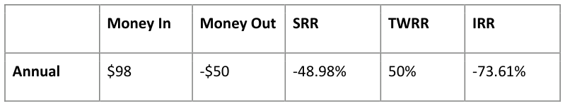
Thus, the three return calculations above produce very different results. The SRR does an adequate but incomplete job of expressing how much money was lost. The TWRR shows performance of the two subperiods, but ignores the differences in the money invested and thus dramatically misrepresents the economic reality to the investor. Finally, the IRR shows the returns actually experienced for each dollar invested.

The relationships between the different returns in this example can also reverse. For example, consider an investor that initially invests $100, has a gain of $20 in that subperiod, withdraws $90, and then ends up with a final value of $24. The returns work out as follows:

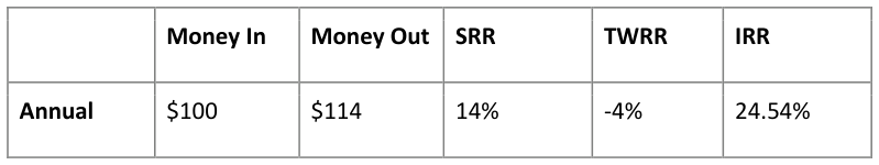
Thus, in this example, the TWRR is negative, while the investor ultimately receives more money than was initially invested, having a SRR of 14% and an IRR of 24.54%.

Perhaps more pertinent to our partners, consider the situation where an investor adds more money as prices drop, making use of dollar cost averaging. Fortunately, we can draw from actual experience in this case! In 2016, one of our partners initially contributed $100,000 for Q1. As partners may recall, our return for that quarter was -12.85%. At our annual meeting and in a note before Q2, we indicated that we believed very good returns could be achieved for any incoming money. This partner then decided to contribute an additional $40,000 for Q2. Subsequent to Q2, our returns for 2016 were 42.43%. Here are the returns with and without this second addition, for comparison:

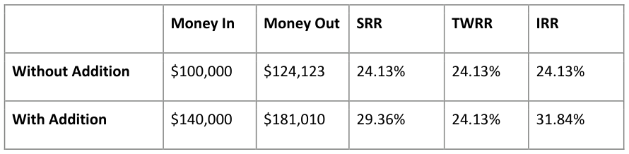
Thus, without averaging down, the partner’s three returns are exactly the same, as there are no cash flows beyond the initial investment. Additionally, in the returns with the addition, the reported performance was also the same as without the addition—24.13%—because TWRR does not depend on the amount of money in each subperiod. In contrast, the SRR increases to 29.36%, which understates the IRR of 31.84%. Thus, because this partner was able to invest additional money at a good time, his economic returns (e.g., IRR of 31.84%) were higher than his reported performance (TWRR of 24.13%). Other partners have also benefited from averaging down in other periods.

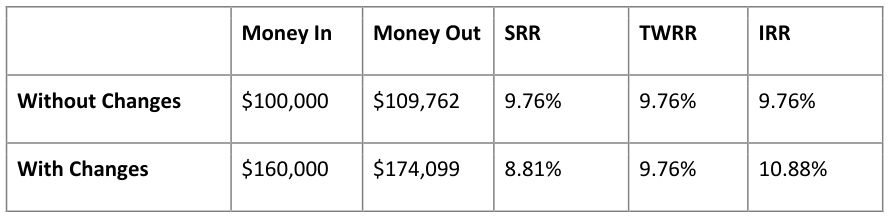
However, not all investors are as contrarian as our partners. A far more common behavior is for investors to become bullish and add money after positive returns and to become pessimistic and withdraw money after negative returns. For example, consider a situation where an investor initially invests $100,000 and Q1 results are positive at 5%. Encouraged, the investor adds another $20,000 for Q2. However, during Q2, a negative macro event happens and equities drop quickly, resulting in a performance of -10%. Worried about this new event and its ramifications, the investor decides to withdraw $40,000 in order to redeploy after the uncertainty has resolved. In Q3, the uncertainty has indeed abated, with returns of 15%. Feeling safer, the investor then adds back the $40,000 he previously withdrew. In the final quarter, the return is 1%, yielding a 9.76% return for the year, which is fairly normal historically. Here are the results with and without this investor’s changes.

Without making any changes, the investor would have had a very decent year of 9.76%. However, with the changes, despite the reported performance remaining exactly the same, the investor’s economic outcome is dramatically worse—having a SRR of 3.84% and an IRR of 4.41%. While this example is perhaps somewhat exaggerated, it is representative. For example, according to Morningstar, the average investor underperforms the funds he is invested in by 1-3% a year, which is a high percentage of returns to lose!

As a final example, consider the exact same situation as above, except that the investor simply adds $20,000 each quarter, ignoring the market’s volatility. Here are how those returns work out:

In this case, the investor has a better economic return than he would have with no changes, despite the down 10% quarter in the middle of the year. In particular, the SRR is lower due to the cash flows throughout the year (essentially, they are penalized for their shortened investment period), the TWRR remains the same as usual, and the IRR is significantly higher.

Conclusion

Thus, each of these three techniques for calculating returns is useful for different situations. The SRR is convenient in any situation where there are no interim cash flows—just a beginning and ending value. TWRRs and IRRs are used when there are interim cash flows, but serve different purposes. In particular, TWRRs are the industry standard for measuring the performance of investment managers, which is appropriate because managers do not have control over the cash flows of their investors. In contrast, IRRs are useful for investors to measure their true economic returns as well as evaluate whether their cash flows have been helpful or detrimental to their overall performance. Going forward, we will continue to report our performance as a TWRR, but will augment individual statements with an individual IRR.