Cost of Leverage

Before embarking on discussions of leverage, a few disclaimers are in order. First, leverage should be used with extreme caution . Second, my understanding of options is based on my own (and several like- minded people’s) reasoning and intuition and has largely come about from evaluating the merits of TARP (troubled asset relief program) warrants in comparison to other leveraged vehicles, such as options and margin. While I have a basic understanding of Black-Scholes, volatility, and other common concepts in the field, everything discussed here is derived from an application of logic de novo . Thus, many of the ideas presented may be construed as either reinventing the wheel or lacking various principles that experts may view as fundamental to options. Nonetheless, I believe these models are helpful in evaluating different forms of leverage and represent a more intuitive method for selecting among available leveraged investment vehicles.

Investment Vehicles

For any investment, there are a variety of vehicles to choose from. First, there are different levels of capital structure to consider: common shares, preferred shares, or debt, among other more complicated choices. For the purposes of this essay, higher positions in the capital structure are ignored, since the focus is on levered equity investing. Accordingly, the remaining choices are simply buying unlevered common shares or applying leverage to those shares in some form. Generally, leverage can be obtained by borrowing money and purchasing common shares (e.g., by using margin in a brokerage account or borrowing from some other source, such as a home equity loan) or via call options or warrants 1 .

The structures of these leveraged vehicles are somewhat different. For borrowed money, an investor simply pays interest on the loan, usually expressed according to an annual rate, which may be fixed or floating depending on the terms. For calls, an investor pays an up-front sum of money (referred to as the call “premium”) to have the ‘option’ to purchase the underlying stock at a specified price (the “strike price”) within a specified window of time (the “option period”). This premium consists of two different parts, commonly referred to as the call’s “intrinsic value” and “extrinsic value”. The intrinsic value of the call is the amount the current stock price is above the strike price and thus represents the value of the call if it were exercised immediately. If a call is “out of the money”, the current stock price is below the strike price, and the intrinsic value is zero. The extrinsic value is simply the remaining portion and can be determined by taking the difference between the price of the call option and the intrinsic value. For an “out of the money” option, the extrinsic value is the entire option price. Thus, the extrinsic value is the extra amount paid, over and above the intrinsic value, to obtain the right to purchase the underlying stock at the strike price during the option period. The extrinsic value represents the time value of the option.

The forms of the cost incurred for these two types of leverage are quite different. When the leverage is structured as a loan, the cost is the interest rate that is charged to the investor to borrow the money. On the other hand, when the leverage is structured as a call, the cost is the extrinsic value of the call. These two costs are not directly comparable due to differences their respective forms, and in particular structural differences between the two investment vehicles. For example, the extrinsic value of the call is paid upfront, whereas the interest charges on the loan are generally paid over time. Another difference in costs is that the call holder typically does not enjoy the benefits of dividends (although some warrants do have dividend protection), whereas the loan holder does. Finally, for a loan there is additional

1 Collectively referred to as “calls” for the remainder of the essay.

downside exposure beyond the interest cost because additional loss is incurred when the stock price falls below the purchase price. In contrast, the only money at risk for a call is the initial cost of the call. In other words, the loan is recourse in nature whereas the call is nonrecourse .

As a concrete example, consider a stock having a share price of $10 and paying an annual dividend of $0.25. An investor might be able to purchase a call expiring in a year and having a strike price of $10 (and thus having no intrinsic value) by paying $1.00 upfront. Alternatively, the investor might instead take out a loan to borrow $10 to purchase the share, but pay $0.50 in interest costs over the course of the year. While it may initially appear that the loan is cheaper than the call, these two costs ($1.00 and $0.50, respectively) are not directly comparable for the reasons identified above. First, the $1.00 premium understates the expense relative to the $0.50 interest cost because it is paid upfront whereas the $0.50 in interest is paid over time. Second, the loan holder’s cost is reduced by the $0.25 dividend whereas the call purchaser’s cost is not. Finally, and more importantly, the downside of the loan is much higher than the call. More specifically, with the call, the purchaser can only lose the initial $1.00 if the stock price at expiry is $10 or less. Thus, the call purchaser is effectively borrowing $10 to purchase a share of the company, but only has $1.00 of loss exposure. On the other hand, the loan holder is actually borrowing $10 and is potentially liable for the entire loan amount, i.e., he could potentially lose much more than the $0.50 in interest costs. For example, in the extreme case where the stock price goes to $0 at the end of the year, the call purchaser does not owe anything and has only lost the initial $1. In contrast, the loan holder would pay the $0.50 in interest costs, receive the $0.25 dividend, and would end up repaying the full $10 loan. Accordingly, in this worst-case scenario, the call purchaser loses $1 while the loan holder loses $10.25. Thus, the apparent high cost of the call was more than offset by its nonrecourse nature.

In order to assess the relative merit of these two vehicles, the costs for each vehicle need to be adjusted to enable a direct and meaningful comparison. In particular: 1) the cost of the call must be adjusted to account for the time value of the up-front payment; 2) the cost of the call must be adjusted to include the value of any missed dividends; and 3) the cost of the loan must be adjusted to include an amount of downside protection comparable to that of a call (e.g., via purchasing insurance such as a put). By making these adjustments, a “Cost of Leverage” may be derived for each vehicle, which can be directly compared in an “apples to apples” manner. The following sections detail these derivations, provide illustrative examples, and discuss how Cost of Leverage calculations can be used to more intelligently compare these different leveraged investment vehicles.

Calculating Cost of Leverage without a Dividend

Since dividends introduce a fair amount of complexity, it is easiest to begin calculating the Cost of Leverage by initially considering stocks that do not include them. As a value investor, my go-to example stock is Berkshire Hathaway, which does not pay a dividend. On June 24, 2016 (Brexit Day), BRK-B had a stock price of $139.71. For simplicity, in this example the Cost of Leverage calculations use virtually at the money puts and calls, having strike prices of $140 (ignoring the $0.29 difference).

Loan Cost of Leverage Calculation

As noted above, in order to provide a directly comparable “Cost of Leverage” between a loan and a call, the loan must be adjusted to include downside protection comparable to the call under consideration. The easiest way to obtain that downside protection is to purchase a put with a same strike price as the call, which provides downside protection from loss beyond that strike price. Thus, the Cost of Leverage for the loan is the total interest cost plus the total put cost. Because investment size and periods for the two vehicles may differ, it is convenient to express the Cost of Leverage in an annualized percentage

format. Accordingly, the annualized Cost of Leverage (CoL) for a loan is relatively straightforward and can be calculated as follows:

Loan CoL= Annual Interest Cost+ Annual Put Cost

Using Interactive Brokers as a reference point for typical margin interest, a small margin loan has an annual interest cost of 1.5% over the benchmark rate, which currently sums to 1.89%.

The price of a put having a strike price of $140 and expiring on January 20, 2017 is $7.20. To calculate the annualized cost of the put, we can use the following formula:

365 number of days ⁄

Annual Put Cost= (1 + Put Price Strike Price−Put Price )

In the first portion of the above formula, the overall put cost is $7.20 / ($140 - $7.20), which is 5.42%; however, this number needs to be annualized. The number of days from June 24, 2016 to January 20, 2017 is 210 days. Thus, the resulting calculation is:

Annual Put Cost= (1 + 7.20 140 −7.20 )

Accordingly, the Annualized Cost of Leverage for the loan is simply:

Loan CoL= 1.89% + 9.61% = 11.5%

Thus, the Cost of Leverage for the loan, with the downside protection provided by the put, is 11.5%.

Call Cost of Leverage Calculation

The Cost of Leverage calculation for calls is a bit more complicated, at least conceptually. A common approach to calculating the equivalent borrowing cost of a call is to conceptualize the extrinsic value of the call as an interest cost and the strike price as the borrowed amount, which can then be used to derive a percentage cost of the effective loan. However, the main issue with this approach is that it ignores the prepaid nature of the interest cost—that is, rather than the extrinsic value being paid over time as interest is in a typical loan, it is paid upfront. Said another way, because the interest is paid all at once at the outset instead of over time, the amount being effectively borrowed is lower than it seems. In actuality, the strike price is not the true “borrowed amount”. Rather, the call investor is purchasing exposure to a common share by paying the price of the call and thus the difference between the share price and the call price is borrowed rather than the strike price. Accordingly, the Cost of Leverage formula for the call can be expressed as follows:

Unannualized Call Cost of Leverage= Interest Borrowed Amount = Extrinsic Value Stock Price−Call Price

The extrinsic value can be found by subtracting the stock price from the sum of the price of the call and the strike price. As a result, the unannualized Cost of Leverage for the call can be fully expressed as:

Unannualized Call Cost of Leverage= Call Price+ Strike Price−Stock Price

Stock Price−Call Price

This formula can be adapted to include the annualized Cost of Leverage as follows:

(Stock Price−Call Price) ∗(1 + Call CoL) % of year = Strike Price

Turning back to our example stock, on June 24, Berkshire Hathaway had a stock price of $139.71, and a $140 call, expiring on January 20, 2017, cost $8.45. Putting these values into the formula gives:

($139.71 −$8.45) ∗(1 + Call CoL)

Solving for Cost of Leverage gives 11.78%. Thus, Costs of Leverage of the loan and the call turn out to be very similar, which makes sense, as otherwise someone could potentially go long one vehicle and then short the other in order to make the spread (though such an arbitrage may still be subject to certain risks, such as changing interest rates).

A Different Conceptualization of Cost of Leverage

The Cost of Leverage can also be conceptualized in an entirely different way. Without any leverage, the investor’s return would simply be the return of the common shares over the same time period. Accordingly, when using leverage the return on investment must be greater than the common return in order for the leverage to have been worth the risk. In other words, if the return using the leverage is less than what would have been obtained without taking leverage at all, then the cost of that leverage was too high ! Using this different model for the Cost of Leverage, the formula for the loan Cost of Leverage remains exactly the same, since the two costs that are incurred due to using the leverage are simply the cost of the interest and the put, which would not have been paid if the leverage were not taken. However, for the call Cost of Leverage, an entirely different, but equivalent, formula can be used. First, the returns of each of the common and call need to be determined at a future stock price, as follows:

Common Return= Future Stock Price

Current Stock Price

Call Return= Future Stock Price−Strike Price

Current Call Price

With this new model, the call Cost of Leverage can be calculated from the future stock price where the return of the common and the call are the same. This “break-over” point 2 can be determined by setting the two equations above equal to each other and solving for the future stock price, which represents the hypothetical future stock price at which the two vehicles would give the same return. This exercise yields the following formula for the break-over future stock price:

Future Stock Price= Stock Price∗Strike Price

Stock Price−Call Price

Then, the call Cost of Leverage can be calculated by determining the annual growth required to reach the future stock price from the current stock price. Following the Berkshire example above, using this equation the break-over future stock price is:

Future Stock Price= $139.71 ∗$140

$139.71 −$8.45 = $149.01

This future stock price of $149.01 requires an annual rate of appreciation of 11.78%, thus giving the exact same Cost of Leverage as the earlier formula.

2 There are two main price points used when discussing calls: 1) the “in the money” point where the call has any intrinsic value, and 2) the “break-even” point where the intrinsic value of the call is equal to the initial cost of the call. However, there is no term for the point discussed in this essay, which I have dubbed the “break-over” point (although I am also open to the “Stevens” point).

Calculating Cost of Leverage with a Dividend

Things change somewhat when the underlying stock pays a dividend. On the loan side, there is no extra cost since the dividend is paid on the borrowed shares. However, for the call, unless there is some form of dividend protection (which is rare) things become a little more complicated, and the Cost of Leverage becomes an estimation since the exact value of future dividends cannot be known. There are a number of possible ways to approach calculating the call Cost of Leverage when the underlying stock pays a dividend, several of which are presented in this section.

First Approach

One approach in factoring in the missed dividends is to simply add the estimated cumulative missed dividends over the period of the call to the total return of the stock. Using the future stock price break- over approach above, the formulas for the future returns of the stock and the call, including dividends, are:

Total Common Return= Future Stock Price+ Cumulative Dividends

Current Stock Price

Call Return= Future Stock Price−Strike Price

Current Call Price

Similar to above, the break-over point can be determined by setting these two equations equal to each other and solving for the future stock price (where the two vehicles would give the same return). This exercise yields the following formula for the break-over future stock price:

Future Stock Price= Stock Price∗Strike Price+ Dividends∗Call Price

Stock Price−Call Price

This break-over future stock price can be used to derive the call Cost of Leverage as discussed above. As an example, consider the GM B warrants. Unlike almost all of the other TARP warrants, these have no quarterly dividend protection, and so all of the missed dividends increase the Cost of Leverage of the warrants. These warrants have an expiry date of July 10, 2019 with a strike price of $18.33. The stock price on August 5, 2016 was $30.72 and the warrant price was $13.15. In addition, in 2016, GM paid out a quarterly dividend of $0.38 per share. Assuming the dividend will not increase (which is probably unlikely and thus will likely result in an underestimation of the Cost of Leverage), the cumulative missed dividends will be $4.56. Plugging this into the formula produces the following result:

Future Stock Price= $30.72 ∗$18.33 + $4.56 ∗$13.15

$30.72 −$13.15 = $35.46

Note that there are two different values that can be calculated from this future stock price: the total return (of either the common or the call) and the common stock appreciation required to achieve that total return (the “required common stock appreciation”). The total return is the return that will be gained by both the common and the call at the calculated future stock price. Using the common return formula (although the call return would provide the same result), the total return is calculated as:

Total Common Return= $35.46 + $4.56

Annualizing this total return produces 9.21%, which is the Cost of Leverage for the GM warrants. The required common stock appreciation can also be calculated by simply using the determined future stock price, as follows:

Required Common Stock Appreciation= $35.46

Annualizing this common return results in 4.9%. Thus, if the common stock appreciates by 4.9% annually, both the common and the warrant will yield the same 9.21% annual total return.

Second Approach

An issue with this first approach is that it simply assumes that the dividends are received all at once at the very end of the holding period. Obviously, this is not the case. Because they are received over time and there is value in receiving them before the period is completed, the first approach underestimates their cost. One very simple approach to attempt to remedy this issue is to take the call Cost of Leverage ignoring the missed dividends and then add an annualized dividend cost to that result. Using the GM example and ignoring the dividend gives a Cost of Leverage of 1.42%. A simple cost of the dividend can be calculated using the following formula:

Annual Cost of Dividend= Annual Dividend

Strike Price

Accordingly, using the GM example, the Annual Cost of Dividend is:

Annual Cost of Dividend= $0.38 ∗4

Thus, the call Cost of Leverage can be calculated by adding these two costs together, which is 9.71%. This number is slightly higher than the 9.21% calculated above because the value of the missed dividends are accounted for every year, instead of simply being added at the end, as in the first approach.

Third Approach

A more complex approach to attempt to take into account the value of the missed dividends, including their time value, is to effectively simulate reinvestment of the dividends throughout the investment period. In this third approach, the strike price is assumed to compound at the Annual Cost of Dividend (CoD) rate, which gives the following formula:

(Stock Price−Call Price) ∗(1 + Call CoL) % of year = Strike Price∗(1 + CoD) % of year

Using the GM example, this works out as follows:

($30.72 −$13.15) ∗(1 + Call CoL) 3 = $18.33 ∗(1 + 8.29%) 3

Solving for the call Cost of Leverage gives 9.83%. This third approach is very close to the second approach, and gives a fairly good approximation for the call Cost of Leverage. However, this approach still is not completely accurate. In particular, the value of dividend reinvestment depends on the stock price at the time the dividend is paid, so even this third approach cannot be entirely accurate as the price of the common stock at the time of each dividend cannot be known. Additionally, as previously discussed, the amount of the actual future dividends cannot be known with certainty in advance. However, this

approach is certainly sufficient for evaluating the relative merits of obtaining leverage using calls versus a loan.

Comparison to Loan

Having calculated the Cost of Leverage for the GM warrants including dividends, it is worth considering an equivalent purchase of the common stock using a loan for comparison. As noted above, in order for the Cost of Leverage of the loan to be comparable to that of the warrants, it must be structured in a similar manner. For the GM warrants, the investor has $12.39 in equity and effectively borrows $18.33. Thus, for a comparable loan, for each share, the investor invests $12.39 and borrows the remaining amount - $18.33. Additionally, the risk associated with this borrowed amount is offset by purchasing a put for that amount. The put has a strike price of $18, which is the closest available price to the strike price of $18.33 for the GM warrants.

The formula for Cost of Leverage for the loan remains the same, which is simply the annual interest cost plus the annual put cost. The annual interest cost is the same as above, 1.89%. For GM, an $18 put expiring on January 19, 2018, costs $0.80 (noting that this expiry date is much earlier than the GM warrant expiry, but is the longest available). Plugging this into the annual put cost formula above gives an annual put cost of 2.72%. Adding these two together gives a Cost of Leverage of 4.61%. In this case, it is clear that the Cost of Leverage is substantially higher for the warrants than for the loan. Almost all of this difference is due to the dividends themselves. As noted above, the cost due to non-receipt of the dividends alone is approximately 8.3%. The Cost of Leverage of the warrants cannot fall below this cost of dividends because, if it did, the intrinsic value of the warrant would exceed the cost of the warrant, which would immediately be arbitraged away (i.e., by buying the warrant and immediately exercising it for a profit). Thus, due to the high value of the unprotected dividends and the low strike price relative to the dividends, the GM warrants are structurally disadvantaged compared to the loan.

Interestingly, for GM, a near the money put expiring on January 19, 2018, costs $4.30. Plugging this into the annual put cost formula above gives an annual put cost of 10.3% and adding this cost to the annual interest cost gives a Cost of Leverage of 12.2%. Thus, a leveraged investment in the common using a loan can be made for almost the same Cost of Leverage as the GM warrants, with downside protection for the full share amount rather than just the loan amount.

Relationship Between Cost of Leverage and Percent of the Money

Cost of Leverage can vary quite dramatically over time based on a wide variety of factors, such as volatility of the common shares, current implied volatility, expected future returns, etc. One of the strongest predictors of the Cost of Leverage is the degree to which the option (i.e., the call or the put, depending on the vehicle type) is in or out of the money. For simplicity, a single term “percent of the money” is used, which is the ratio between the stock price and the strike price, subtracting 1 in order to normalize it around 0. For example, when the price of stock is $10, a $5 strike price call is 50% “of the money”. For the same stock, a $15 strike price call is -33% “of the money”.

Intuitively, this percent of the money relationship makes sense—the deeper in the money a call is, the more it resembles the common shares. After all, a common share is nothing more than a 100% in the money call. Similarly, as the put gets further and further below the current strike price, it provides less and less insurance for a downturn, and therefore becomes less expensive.

However, as shown above the Cost of Leverage can also be heavily influenced by dividends, potentially providing a floor under which the Cost of Leverage cannot fall. For example, as shown for GM warrants, the Cost of Leverage cannot fall below 8.3% per annum. In order to better examine the general relationship of Cost of Leverage and percent of the money of the warrant, the following discussion excludes the value of missed dividends as a factor, which tends to obscure the relationship. However, this exclusion can be easily compensated for, after-the-fact, by adding the dividend cost to the calculated values (i.e., following the second approach discussed above). Thus, this two-step approach (examining the relationship before dividends and then adjusting for the dividends afterwards) allows for a more complete understanding of the development of Cost of Leverage.

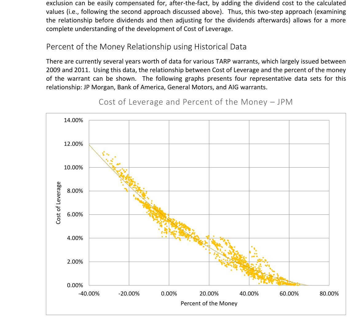
As shown, the JP Morgan warrants show a strong relationship between Cost of Leverage and percent of the money. More specifically, as the warrant percent of the money increases, the associated Cost of Leverage decreases. While initially appearing linear, the slope flattens as the warrant becomes more in the money. This behavior makes intuitive sense because the Cost of Leverage cannot fall below 0 due to arbitrage and must therefore approach it asymptotically.

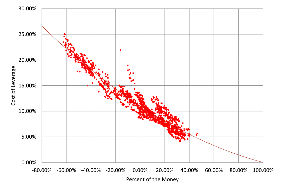
Similar to JPM, there is also a strong relationship between Cost of Leverage and percent of the money for Bank of America A warrants. Of note, BAC’s Cost of Leverage is quite a bit more expensive than JPM’s, overall.

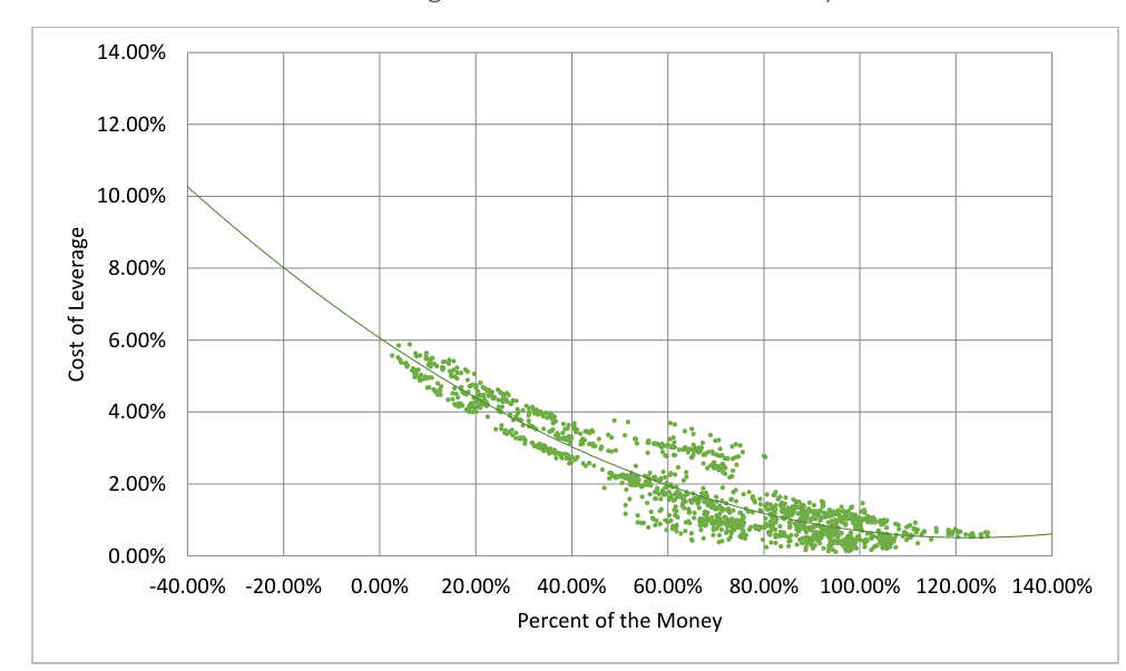
General Motors also shows a strong relationship between the two variables. Note that the GM warrants were never out of the money, so GM shows how the relationship between the two evolves while the warrants are increasingly in the money. In particular, the slope of the line decreases until it asymptotically approaches 0% or just above. However, note that if the dividends were included, this bottom would be the one imposed by the dividends themselves. More specifically, for GM, the graph would have a very similar shape, but the Cost of Leverage would asymptotically approach 8.3% rather than 0%. Similar adjustments apply to the other warrants, except most of these include a dividend adjustment feature at a threshold, e.g., (i.e., $0.01 per quarter for BAC warrants, $0.38 per quarter for JPM warrants, and $0.17 per quarter for AIG warrants). As a result, the floor for these warrants would be set at the annual dividend adjustment threshold rather than the full dividend.

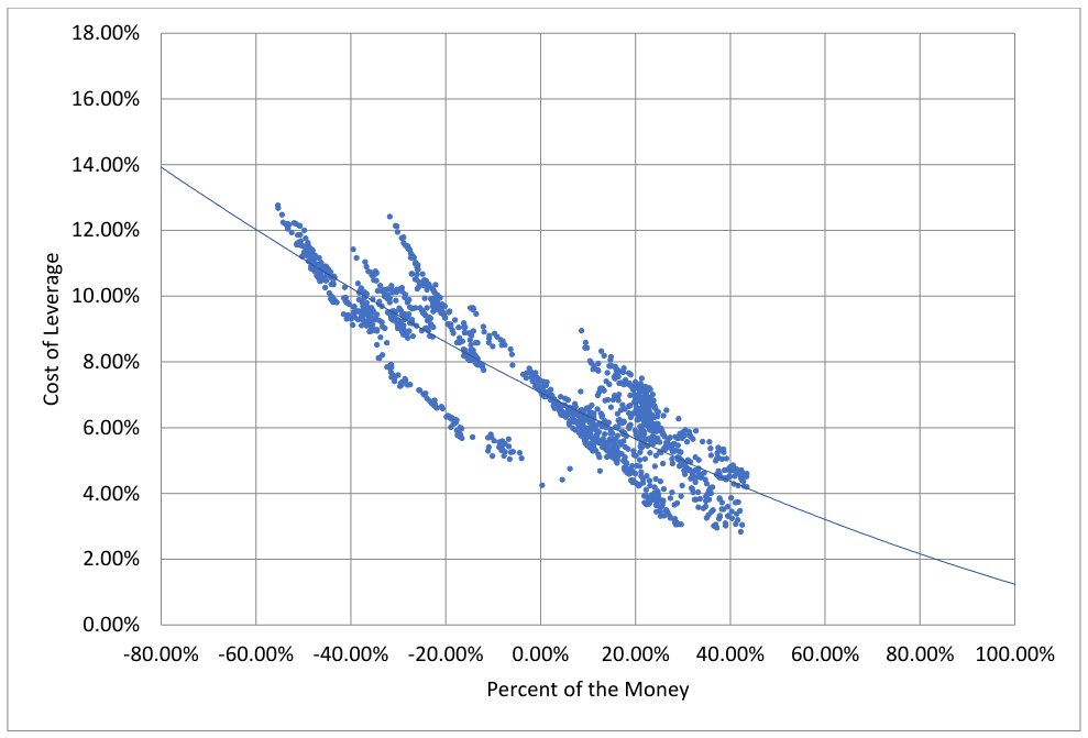
Of the four data sets, AIG has the least correlation between the two variables. Nonetheless, it is clear that as the warrant becomes more in the money, the Cost of Leverage decreases.

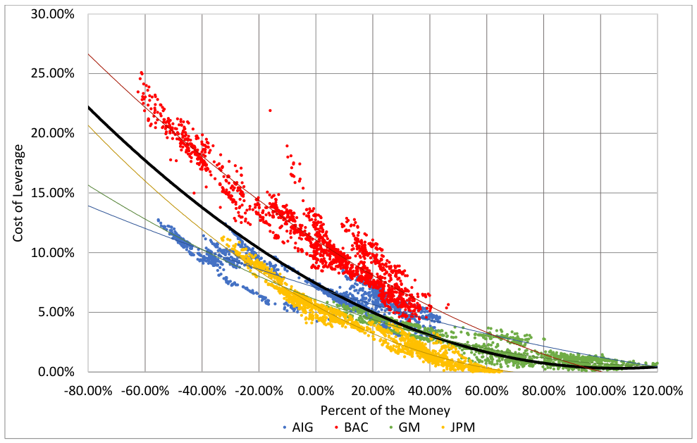
Plotting all of these data sets together, it is clear that even though the relationships between Cost of Leverage and percent of the money are similar, the individual trend lines differ from each other. For example, the Bank of America warrants are routinely more expensive than the JP Morgan warrants at similar levels of percent of the money. In contrast, AIG has been cheaper or more expensive than the JPM warrants at different times. At comparable levels, the General Motors warrants tend to fall in between the JPM and BAC warrants.

The overall trend line, shown in black, represents the general relationship fairly well. However, while it is increasingly representative of the data as the warrants get more in the money, it is not terribly predictive for individual stocks when the warrants are out of the money. As a result, it may be the case that the overall trend line is not particularly useful for evaluating the merits of leverage for individual companies due to their own idiosyncrasies (e.g., their volatility, expected future returns, etc.). On the other hand, it may be possible to draw some conclusions about individual warrants depending on their relative position to this overall trend line (or a better one), discussed below.

Comparing Historical Common and Warrant Returns

Based on the historical return data discussed above, the warrant and common returns for each of these companies have had different outcomes. For each of these companies, the following graphs provide the returns of the warrants and the common as well as the Cost of Leverage of the warrants. More specifically, at each date on the x axis, the blue lines represent the future returns of the warrants to August 2016 if bought on that day (using the left-hand y axis), the red lines represent the same future returns of the

common without taking into account dividends (using the left-hand y axis), and the dotted grey lines represents the Cost of Leverage (using the right-hand y axis).

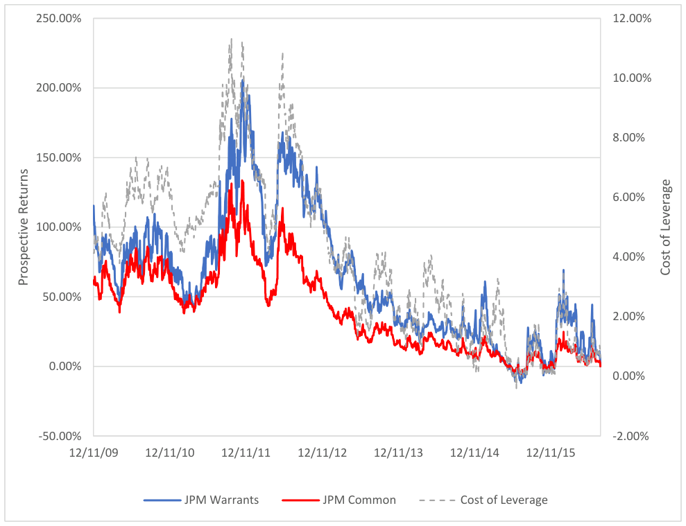
For JP Morgan, the warrants outperformed the common at almost any buying point in the past six years. Additionally, the Cost of Leverage largely tracked the prospective returns. This tracking behavior makes sense because future returns increase as the price decreases, assuming an eventual recovery. At the same time, a drop in price means that the warrant is less in the money, which as shown above, results in a higher Cost of Leverage. For example, at September 22, 2011, the JPM common closed at $29.27 and the JPM warrants closed at $9.24, having a Cost of Leverage (without dividend) of 11.14%, being 31% out of the money. By March 26, 2012, the common had recovered to $46.17 with the warrants at $14.00, having a Cost of Leverage of 4.28% and being in the money 8.84%. Thus, as the prospective returns for the common decreased from 126.51% to 43.6%, the Cost of Leverage also decreased from 11.14% to 4.28%.

An interesting observation is that the JPM warrants were “cheaper” overall on a Cost of Leverage basis than almost any of the other warrants, as shown in the overall chart above. Thus, it is not surprising that JPM warrants, as the lowest Cost of Leverage warrant, generally outperformed the common throughout its history. Said another way, because almost every data point of the JPM Cost of Leverage fell below the overall trend line, it is not that surprising that the JPM warrants outperformed the common shares.

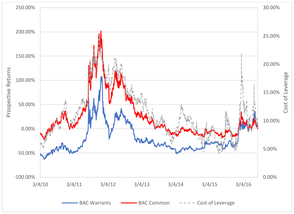
Bank of America shows exactly the opposite relationship between the common and warrant performance than that of JP Morgan. As shown, assuming a holding period until August 2016, the BAC common almost always outperformed the BAC A warrants. The Cost of Leverage varied with prospective returns in a manner similar to the JPM warrants, though at a universally more expensive level.

Following the observation above for JPM warrants, the BAC warrants Cost of Leverage was always more expensive than the overall trend line. Thus, it appears that this high Cost of Leverage provided a headwind too difficult for the warrants to overcome throughout their history.

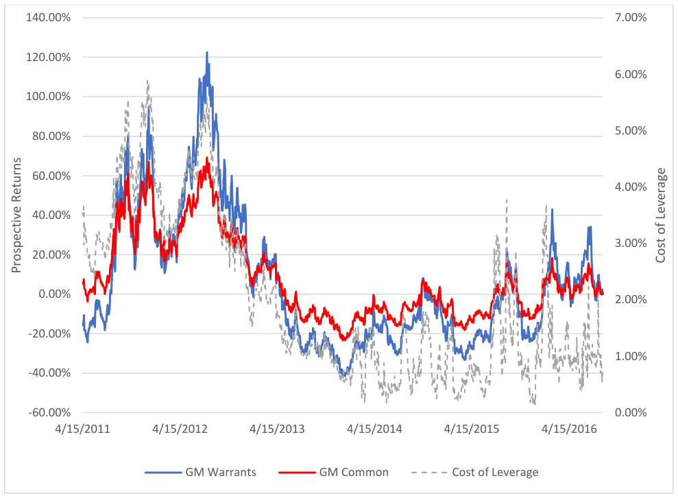
For General Motors, the best returns alternated between the B warrants and the common at various points in time. Similar to the previously discussed warrants, the Cost of Leverage varied with the prospective returns, showing quite a bit of volatility from 2014 to 2016.

In the overall graph previously shown, data points for the GM warrants largely fell on the trend line, though perhaps with some skewing below the trend line when near the money and above the trend line when deep in the money. This skewing correlates somewhat well to the outperformance and underperformance of the warrants shown in the present graph.

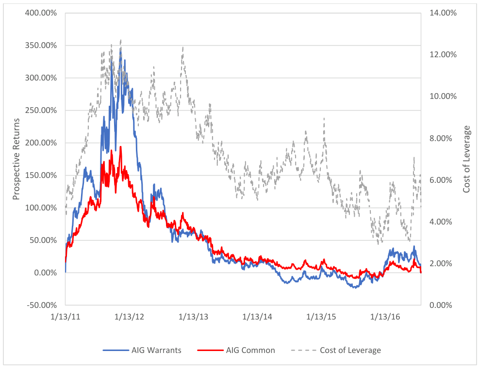
AIG largely shows two different regimes, an initial period where the warrants outperformed the common, and a longer later period where the common was generally better than the warrants. This two-period behavior appears to correlate well to the periods of time when AIG was above and below trend line shown in the overall chart. More specifically, in the earlier period, the warrants were out of the money, corresponding to data points falling below the overall trend line. As the warrants changed to being in the money, the Cost of Leverage began to go above the overall trend line. At the same time, the warrants began to underperform the common, as shown above.

AIG also shows a different Cost of Leverage development, initially following the same pattern as the previous companies, but generally staying higher throughout the second period than might normally be expected. It is not immediately clear why AIG developed in this anomalous manner.

Warrant Returns and Changing Cost of Leverage

Generally, the point of purchasing a warrant is to obtain leverage—ideally achieving a higher gain than would have been obtained by simply buying the common shares in an unlevered manner. Assuming a constant Cost of Leverage and an increasing common share price, this is exactly the outcome that would be achieved. However, the Cost of Leverage does not behave in this manner. As shown above, the Cost of Leverage generally decreases until a floor is reached as the warrant gets deeper in the money. On the

other side, as the warrant gets more out of the money, the Cost of Leverage increases. Thus, Cost of Leverage changes inversely with stock appreciation. Accordingly, because of the countervailing force of the changing Cost of Leverage, the actual experienced leverage is much less than might intuitively be expected. By examining the BAC historical returns over three distinct periods, this phenomenon can be shown explicitly.

BAC Prospective Returns – 3/4/10-12/19/11

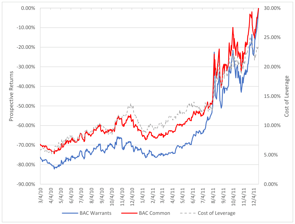
The BAC A warrants began trading on March 4, 2010. On that date, the BAC common had a price of $16.40, and the BAC A warrants had a price of $8.41 with a Cost of Leverage of 5.91%, excluding the effects of dividends. By December 19, 2011, the BAC common had decreased to a low of $4.99, and the BAC A warrants had a price of $2.00 with a Cost of Leverage of 23.86%. Over this period, unsurprisingly, the BAC A warrants experienced worse losses than the common, but the difference in those losses were fairly small. More specifically, over the entire period, the BAC common experienced a loss of 69.6% and the BAC A warrants experienced a loss of 76.22%, a difference of only 6.62%. However, had the Cost of Leverage remained at 5.91%, the BAC A warrants would have been priced at an impossible -$3.86. Alternatively, had the Cost of Leverage initially been 15%, the initial warrant price would have been $12.55, and the final warrant price would have been $0.06, experiencing an almost 100% loss over the period. Thus, the increasing Cost of Leverage of the BAC A warrant over this period virtually erased the leveraging effect of the warrant entirely . Said another way, the increasing Cost of Leverage largely mitigated the leverage provided by the warrant, resulting in returns essentially the same as the common.

BAC Prospective Returns – 12/20/11-7/22/15

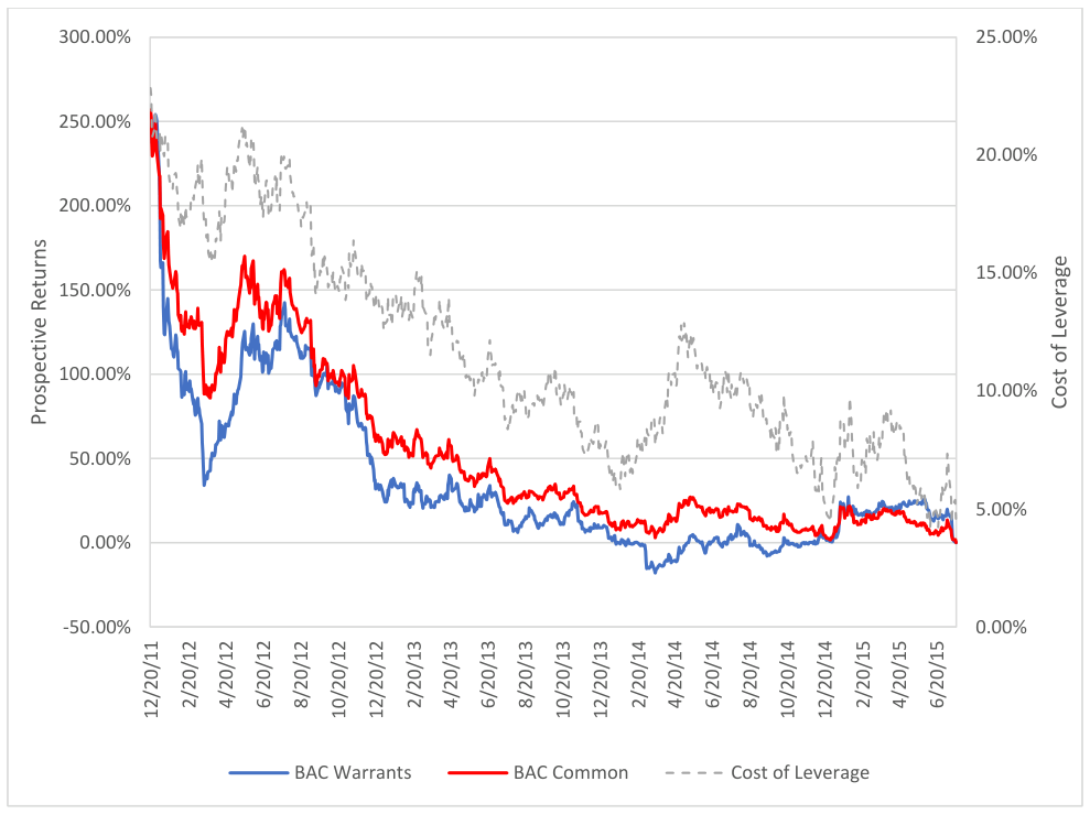
In the next period, to July 22, 2015, the BAC common increased from its low to $18.45. Similarly, the BAC A warrants increased to $7.08, while the Cost of Leverage decreased to 4.59%. Incredibly, throughout this astounding price rise, the BAC A warrants were almost never the better choice, even though they supposedly provided leveraged upside. For example, over the entire period, the BAC common experienced a gain of 256.87% while the BAC A warrants experienced a gain of 242.03%. In contrast, had the Cost of Leverage stayed constant at 23.86%, the BAC A warrants would have been priced at $12.15 and had a gain of 487%. Thus, in this second period, the changing Cost of Leverage actually caused the BAC A warrants to have effectively have less leverage than the common .

BAC Prospective Returns – 7/23/15-8/5/16

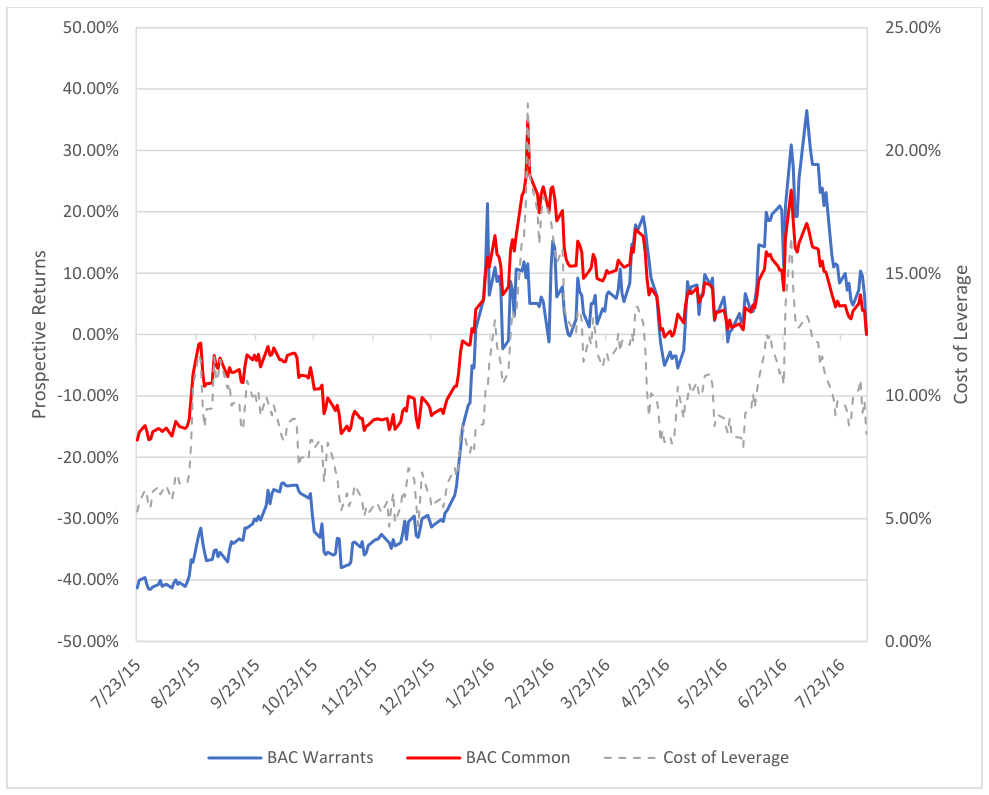
In the final period, to August 5, 2016, the BAC common decreased to $15.05, after having rebounded from a low of $11.16 on February 11, 2016. During this period, the BAC A warrants decreased to $4.15 while the Cost of Leverage almost doubled to 8.46%. In this case, while the change in Cost of Leverage did mitigate the leverage to some extent, over the entire period the BAC A warrants experienced more than double the losses of the common (-41.3% versus -17.22%).

Conclusions

When electing whether and how to take on leverage for an investment, it is obviously important to understand how much that leverage costs, as outlined initially in this essay. However, it may be at least as important to understand how that Cost of Leverage is likely to change throughout the investment.

For example, many value investors examined Bank of America’s situation when the price of its common stock was $5 in 2011 and correctly identified that the common could appreciate more than 3x over 3-5 years. They also identified that the Cost of Leverage was quite high, but naively assumed that because the expected returns were in excess of the Cost of Leverage, the warrant would outperform the common. However, even though the actual return of the common did indeed exceed that initial Cost of Leverage, these investors did not realize higher gains than the common, because of the manner in which the Cost of Leverage decreased as the warrant became increasingly in the money! Sadly, these investors, myself included, did not fully understand how the Cost of Leverage would develop throughout the common share appreciation, and accordingly misjudged the prospective returns of the Bank of America TARP warrants, despite having accurately assessed the prospects of Bank of America and the prospective returns of its common stock. As this example illustrates, a fuller understanding of both the Cost of Leverage and its typical behavior over time can be very helpful in analyzing various vehicles for taking on leverage. Further, such an understanding can, when used in conjunction with sound security analysis, provide a more comprehensive basis for judging the relative prospective returns of various possible levered and unlevered investment vehicles, and, in turn, for choosing whether and with what vehicle to take on leverage.