Why Hold Cash?

Since the bottom of 2009, the S&P 500 has risen almost 200%; the Shiller P/E is ~25, well above its 16.5 historical average; corporate margins are greater than 10%, also well above their 6.5% historical average; the total market capitalization of the U.S. is more than 120% of trailing GDP, greater than the so-called “fair value” of 75%-90%; margin levels have broken new records; and there are a remarkable number of highly priced initial public offerings. Further, from my own experience, even investors that have previously “ignored the macro” increasingly believe that overall market conditions can no longer be overlooked in light of the recent financial crisis. As a result, many are now advocating or are themselves holding larger cash positions as market prices have increased. In order to determine whether this behavior can reasonably produce higher returns, this essay surveys a variety of models and backtests to compare long-term returns among portfolios having different levels of cash.

To be clear, this essay is not focused on whether or not cash should be held in the absence of opportunities that meet minimum investment requirements —I believe that cash should be held in such situations. Instead, this essay addresses whether cash should be held when there are still compelling investments to be made . Additionally, before beginning this essay, I fully expected that at least a 5-10% cash position would be warranted in many environments; however, with a few important qualifications, it appears that holding cash in these situations reduces long-term performance.

Hindsight Models

A natural first test to determine whether holding cash is a viable strategy is to model portfolios under the assumption that cash can be properly deployed after significant price decreases and compare the results of such model portfolios to a fully invested portfolio over the same time period. Similar to previous essays, both the model portfolios and the fully invested portfolio were compared using Shiller’s market data from 1871 to present, on an annual basis. Because some later models use averaged or percentile values from previous years, each comparison is made from 1890 to present, to keep the results comparable across tests.

1 Year Downturn Model Portfolios

In a first set of models, a percentage of cash (that is varied for each member of the set) is assumed to be held in most “normal” years, but is fully invested whenever the annual returns turns negative and when the next year will be positive, thereby guaranteeing that each model portfolio is only fully invested in positive years following negative years (i.e., investing at the bottom of a downturn). In all other years, each portfolio retains its respective percentage of cash, waiting for the next price decline. For example, from 1924-1928, each model portfolio would hold its specified percentage of cash, and would continue to do so from 1929-1932, all of which had negative returns. Then, each model portfolio would be fully invested and take advantage of the 55% total return of 1933. As another example, from 1970-1972, each model portfolio would hold its specified percentage of cash, and would continue to do so through 1973 and 1974, which both had negative returns. Then, each model portfolio would be fully invested and take advantage of the 38.5% total return of 1975. Thus, these models essentially assume perfect timing on deploying cash into the market, on an annual basis.

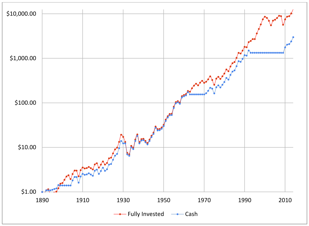
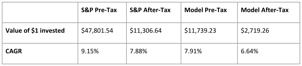
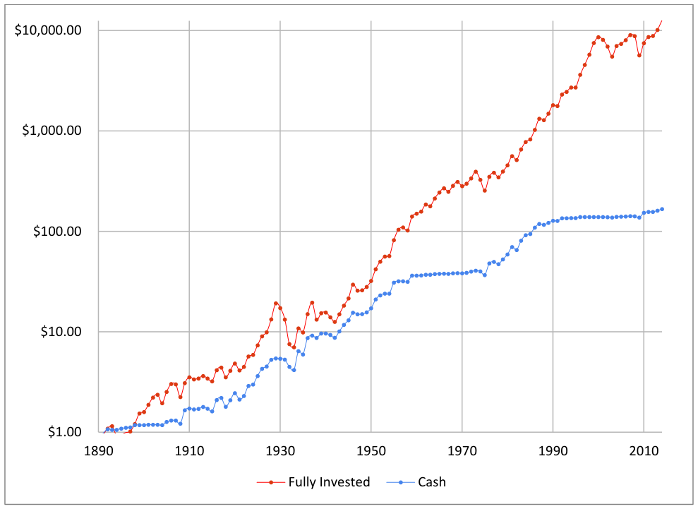
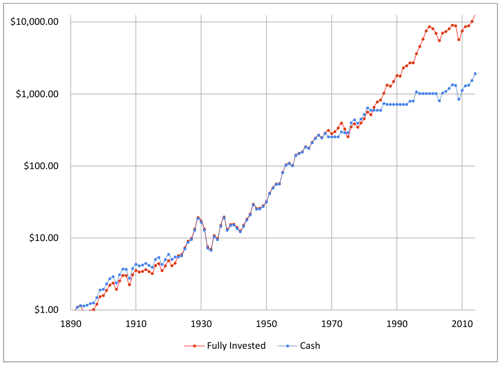
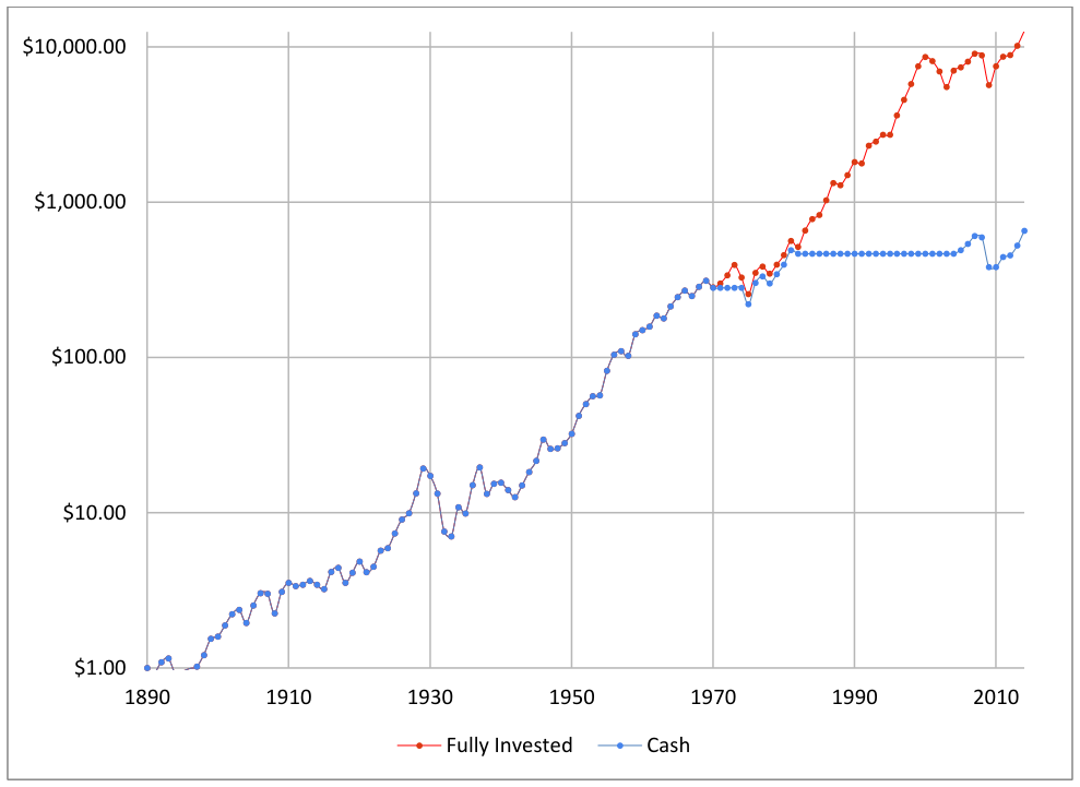
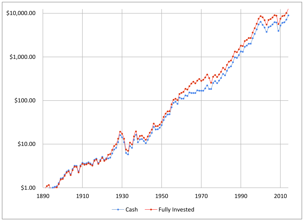
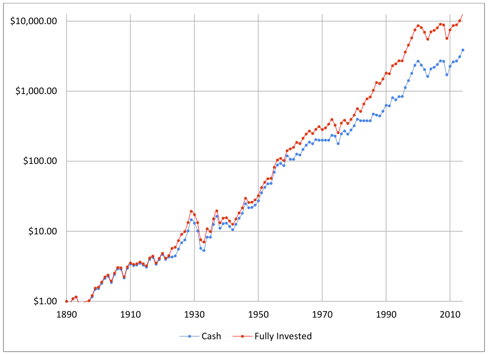
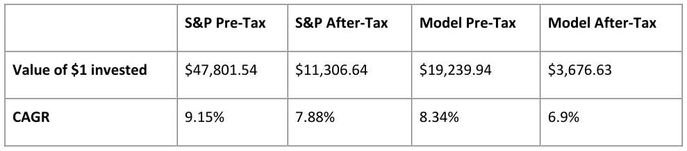
The following graph and table present the comparison of the post-tax returns of the S&P and a model portfolio using a default 10% cash holding over the period from 1891-2014. Assumptions are that dividends and capital gains are taxed at 20%, after-tax dividends are reinvested, and S&P turnover is 4% per annum.

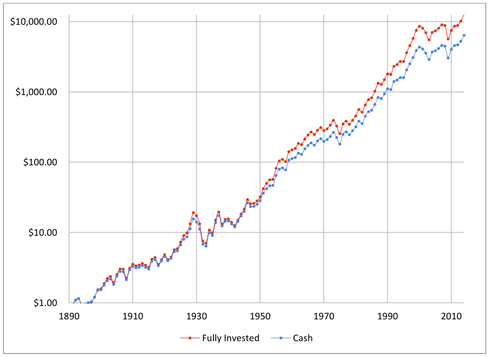
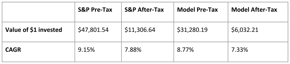
As shown, even assuming perfect timing of investing the cash in the portfolio, the model portfolio underperforms the S&P over the time period. Note that while the results for a default cash percentage of 10% cash portfolio is shown, any cash percentage other than 0 resulted in underperformance, with the degree of underperformance increasing as the cash position increases from 0% to 100%.

3 Year Downturn Model Portfolios

In a second sets of models, a percentage of cash (that is varied for each member of the set) is assumed to be held in most “normal” years, but moved to 100% invested for three years after a downturn. In all other years, each portfolio retains its specified percentage of cash, waiting for the next downturn.

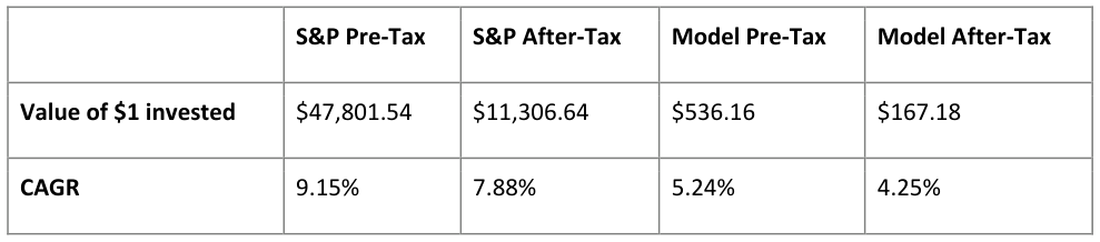
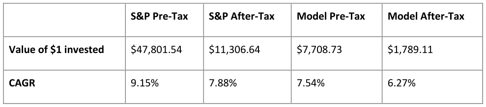
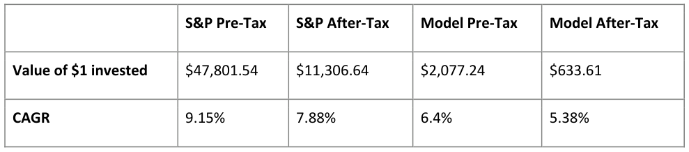
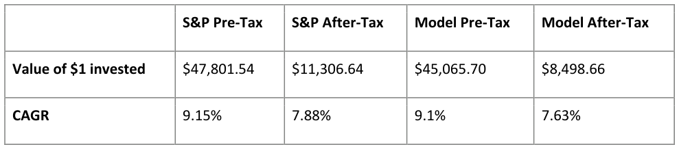
The following graph and table present the comparison of the post-tax returns of the S&P and a model portfolio using a default 10% cash holding over the period from 1891-2014. The same assumptions as previous models are used for dividends, taxation, and turnover.

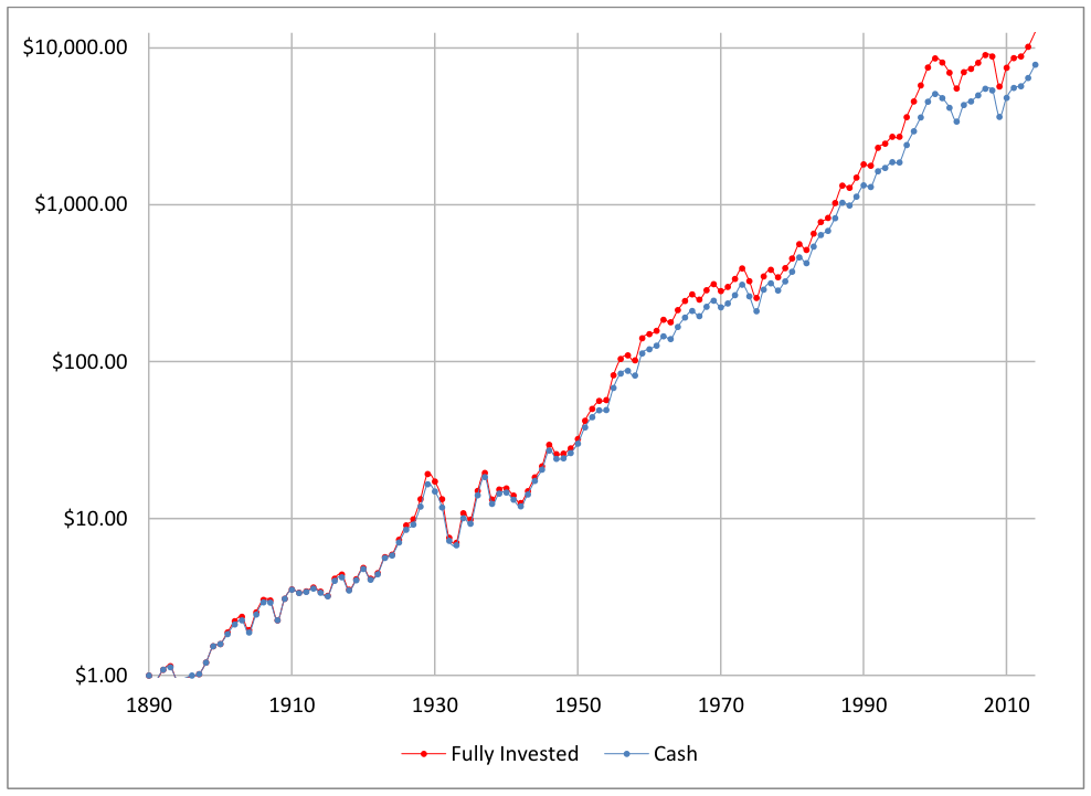
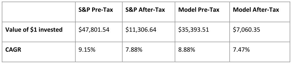
Similar to the previous set of models, note that while the results for a default cash percentage of 10% is shown, any cash percentage other than 0 resulted in underperformance, with the degree of underperformance generally increasing as the cash position increases from 0% to 100%.

Thus, in either set of models, assuming perfect timing for investing the held cash , the fully invested portfolio still provided higher returns. However, if the volatility is increased fairly significantly, a non-zero cash strategy can start to be effective. For example, if the same one year downturn model is used, but the volatility is increased by 100%, holding approximately 6% cash would have provided a higher pre-tax return than not holding cash. Interestingly, however, the after-tax returns are still better with 0% cash held. The following table summarizes these results:

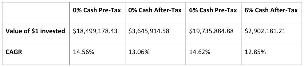
Thus, in this particular model, even when the increased volatility increases the beneficial effect of the cash held (which yields a higher pre-tax return), the tax effects of the increased turnover rate more than offset the additional returns.

Valuation Models

Many investors who advocate holding cash do so based on various valuation models, such as current price- to-earnings ratios, the cyclically adjusted price-to-earnings ratio (CAPE), spreads between stock market earnings yield and treasury rates, etc. Indeed, there are many academic papers indicating that certain strategies outperform the index during a selected sample period, although in almost all cases, the outperformance is on a pre-tax basis. After using several of my own models, and testing those papers that showed outperformance out of their original sample dates, I did not find any reliable method of outperformance. Exemplary results are shown below:

Percentile CAPE Model Portfolios

Many investors rely on the cyclically adjusted price-to-earnings ratio (CAPE) to indicate current market valuation. Indeed, the CAPE value and historical future returns are correlated, and it appears to be usable to provide a reasonable expectation of future returns. For example, the following graph shows the historic relationship between CAPE values and future 10 year returns:

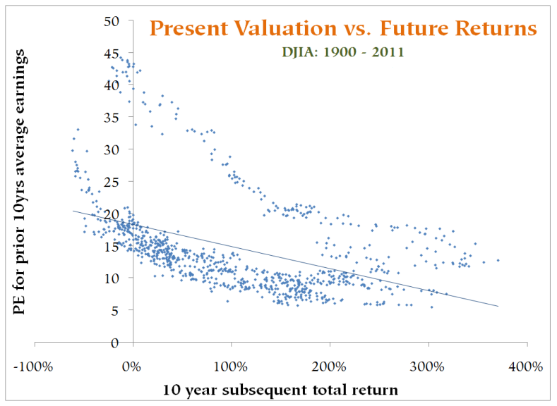
As can be seen, higher CAPE values (shown on the left axis) tend to result in lower 10-year subsequent total returns. From this graph, it is easy to assume that an investor could theoretically stay invested at lower CAPE values and hold cash at higher CAPE values in order to provide outsized returns. However, the data do not bear out this assumption.

For example, consider a CAPE percentile method, where model portfolios are only invested if the current CAPE value is less than a historical n percentile. Thus, each model portfolio stays invested unless the CAPE value indicates overvaluation, depending on a selected value of n . More particularly, where the CAPE value indicates undervaluation, the model portfolio is fully invested, and conversely, where the CAPE value indicates overvaluation, the model portfolio is held entirely in cash. Note that such models avoid hindsight issues by using current percentiles as of each year, rather than a historic percentile, which was unknown at the time.

The following graph and table present the comparison of the post-tax returns of the S&P and a model portfolio using a 90% CAPE percentile from 1891-2014. The same assumptions as previous models are used for dividends, taxation, and turnover.

Similar to previous models, the results get better as the model stays more fully invested.

Variable CAPE Model Portfolio

As another model, rather than the all-or-nothing percentile method in the previous model, a potentially viable alternative is to have a percentage of cash corresponding to the current percentile of CAPE. That is, if the CAPE is at its lowest percentile value, a corresponding low level of cash would be held. Similarly, as the CAPE reaches high percentiles, a higher level of cash is held.

The following graph and table present the comparison of the post-tax returns of the S&P and a model portfolio using the variable CAPE percentile from 1891-2014. The same assumptions as previous models are used for dividends, taxation, and turnover.

Positive 1 Year Spread Model Portfolio

Another technique that has at times been effective and reported in academic papers is based on the spread between the current interest rates and equity earnings yield (i.e., earnings-to-price percentage). In particular, the idea behind this technique is that an investor should invest in equities when the equity earnings yield present a more attractive investment than the yield of the current bond rate. For example, if bond yields are significantly above current equity yields, they may present a better opportunity for the investor. A simple approach is to compare the current earnings yield to the current bond rate, and only invest in the market if the earnings yield is greater. Using the same assumptions as above, the following graph and table illustrate the results using the 1 year treasury yield.

The following graph and table present the results for a positive spread between the earnings yield and the 10 year treasury yield.

Percentile 1 Year Model Portfolios

Rather than simply investing when the spread is positive, another possibility is to compare the current spread to a percentile of differences between the earnings yield and interest rates over a series of years, e.g., avoiding investing when the current spread is in the bottom 5% of recent spreads.

The following graph and chart illustrate the results of using a 95 percentile of spreads for 1 year treasury yields, over a period of 20 years.

Here are the results for the same model, but using the 10 year treasury yield instead of the 1 year treasury yield.

Each model does progressively better the more it is fully invested. It should be noted that the results of the percentile method has shown outperformance, on a pre-tax basis, for the period from 1970-2014. It does not, however, show outperformance over the longer-period in the tests above.

Hypothetical Models

The last two sections essentially boil down to the question of whether or not an investor can “time” the market—given the degree of effort that has already been put into this topic and the immense rewards

that would be reaped by a successful market-timing strategy, I do not think it should be terribly surprising to anyone that there do not appear to be any “easy” answers.

However, the returns for active investors should deviate significantly from market returns. Accordingly, there is the possibility that even if the market as a whole cannot be successfully timed (or at least acknowledging that it is very difficult to do so), it still may make sense for active investors to hold cash, depending on the nature of their returns. In order to address this question, the following models present hypothetical returns and outcomes to determine if and when holding cash can be effective in maximizing returns.

Linear Growth with Bonus Return Model Portfolio

In this model, a linear portfolio (i.e., a portfolio that compounds at a constant rate) is compared against a portfolio that holds a percentage of cash for four years and then invests the cash for a single year in a high return investment, allowing the cash to be deployed very effectively. This model is used as a simplification of Mohnish Pabrai’s current cash holding strategy which operates as follows:

1 st 75% of cash – minimum 2x in 2-3 years next 10% of cash – minimum 3x in 2-3 years next 5% of cash – minimum 4x in 2-3 years next 5% of cash – minimum 5x in 2-3 years last 5% of cash – more than 5x in 2-3 years On its face, this is an elegant strategy for cash allocation. However, it is not clear whether or not it produces better returns than would be gained with a simpler one (e.g., always investing if there is a potential 2x return in 2-3 years). This uncertainty is because it is not known how often these 3x, 4x, 5x, and greater than 5x investment opportunities will occur. If they occur frequently and can be reliably identified, then the strategy will be highly effective. However, if they occur too infrequently and/or cannot be easily identified, the opportunity cost of not investing in lower return opportunities will overwhelm the gains that occur when these extraordinary opportunities arise.

Turning to the simplified model, the linear portfolio simply grows 15% per annum for 22 years. The test portfolio holds a percentage of cash and every 5 th year, invests that cash in a high return investment. It turns out, the “bonus” return that occurs every 5 th year must be approximately 85% or greater in order for holding any amount of cash to begin to be better than the linear model. For a test portfolio where the bonus return occurs every 6 th year, the bonus return has to be 125% or more.

In essence, the bonus return has to more than offset the full five or six years of opportunity cost of the cash portion of the portfolio, which is a high bar to meet at 15% per annum.

Linear Growth with Downturn and Bonus Model Portfolio

As it is highly unlikely that an investor’s portfolio will grow linearly in a consistent fashion as tested in the previous portfolio, and since great investment opportunities tend to occur after or during a downturn, in a further model a fully-invested portfolio grows linearly at 15% per annum, but has a downturn every five years. In the cash portfolio, the cash is held until the downturn occurs, and then invested in a higher return investment opportunity. This model is essentially the same as the previous one, except that the bonus return is earned after a downturn occurs. The downturn is an important modification as it allows the cash to serve two purposes: 1) it does not lose any value during the downturn; and 2) it is invested in a higher-than-normal-return investment.

The results of this comparison are much more palatable. Assuming a downturn of 20% every 5 years, and a bonus return of 25% when the cash is deployed, cash levels of upwards of 50% provide higher returns than 100% invested portfolios. However, if the periodicity of the downturn is extended to 6 years, still assuming a 20% downturn, the bonus return must be 45% or better for any amount of cash to provide higher returns.

Investor Portfolios

While the hypothetical models discussed above do provide some benchmarks for when holding cash can be effective in different scenarios, they are not all that representative of real-life returns. Accordingly, the following models are based on the returns of actual investors, including individual investors, funds, and screens. In these examples, the ex-cash returns were used to create a base model, and varying levels of cash were tested, assuming that the investor would have fully deployed the cash at downturns. In cases where the portfolios were always fully invested, the testing was relatively easy. However, for investors who held cash at various points, the levels of cash were estimated based on information available.

In the following table, the reported returns of the investor portfolios are shown. Additionally, bolded percentages indicate when the cash of the model portfolio was fully deployed. Finally, the ideal cash percentage is shown in the final row.

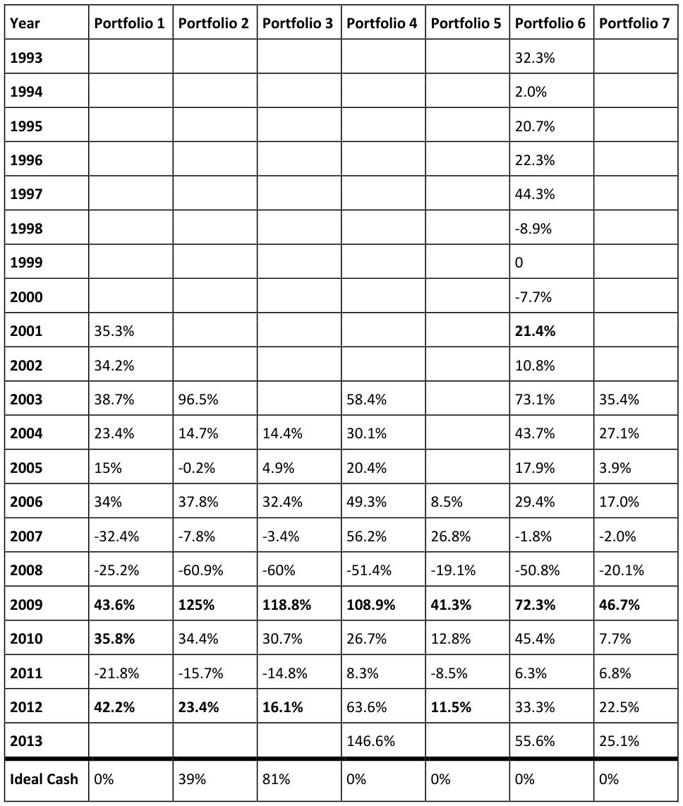
These records are from well-respected, high-performing investors or stock screens. For the most part, it appears that holding cash would not have produced superior returns, except for the case of portfolios 2 and 3. Interestingly, portfolios 2 and 3 are from the same investor as portfolio 1, using the same investments (though having slightly different reporting periods, timing of investments, and proportions). Given the extreme level of volatility and a shorter record in these latter two portfolios, and the fact that the first portfolio did best with no cash over a longer period, I believe that over time the ideal level of cash for these two portfolios will decrease, or even reduce to 0%.

Conclusions

Holding cash appears to be most beneficial for active investors that have extreme volatility (e.g., downturns of greater than 35%) and who are able to deploy the cash at the bottom in extraordinary investment opportunities. For everyone else, however, it does not appear that holding cash provides a superior return to remaining fully invested.

I again emphasize that this essay is not focused on remaining fully invested at all times , but instead advocates remaining fully invested when there are still compelling investments to be made .