The Hurdle for Active Investors

Individuals have two options for investing in equities: passive or active. Active investing involves selection of individual securities with the expectation (or hope) that the investor can beat a market benchmark or index. Passive investing, on the other hand, involves simply replicating an established market index, such as the S&P 500, with the guarantee of achieving market returns. Given the vast number of studies demonstrating that the majority of active investors underperform market returns after fees and expenses, it naturally follows that passive investing should be the default choice. Accordingly, to warrant a deviation from the passive option, an active approach must outperform a passive approach after all costs are taken into account, including transactional fees, management fees, and taxes . Unfortunately, most active investors focus on outperformance on an after—fee, but pre—tax , basis and do not compare their returns to a benchmark after taking into consideration the effects of taxes. When the investment is in a tax—sheltered vehicle such as a 401k or IRA, this attitude may be warranted. For those investments that are not in a tax—sheltered vehicle, however, the effects of taxes must be considered.

The underlying principles for comparing after—tax returns were previously discussed in my prior essay: “Holding Period, Taxes, and Required Performance”. That essay discussed the relationship between holding periods and after—tax returns, in particular the concept that the shorter the average holding period, the greater the number of instances when investment gains are taxed, resulting in lower after— tax returns. This has large implications for the active investor who is investing in a non—tax—advantaged account, since he will have a much higher tax burden than a passive investor.

The present essay applies the principles discussed in that prior “Holding Period” essay to derive the required outperformance that an active investor must achieve to offset his higher tax burden relative to a passive investor. This required outperformance is determined under various scenarios having differences in investment periods, turnover (or inversely, holding periods), and rates of return. Initially, the essay shows various historical returns in order to establish realistic market scenarios. Subsequently, the essay models these scenarios for passive and active investors to provide the hurdle that the active investor must clear, after management fees and costs are taken into account, in order to provide superior returns over the passive investor under each scenario.

Establishing Realistic Scenarios for Passive Investing

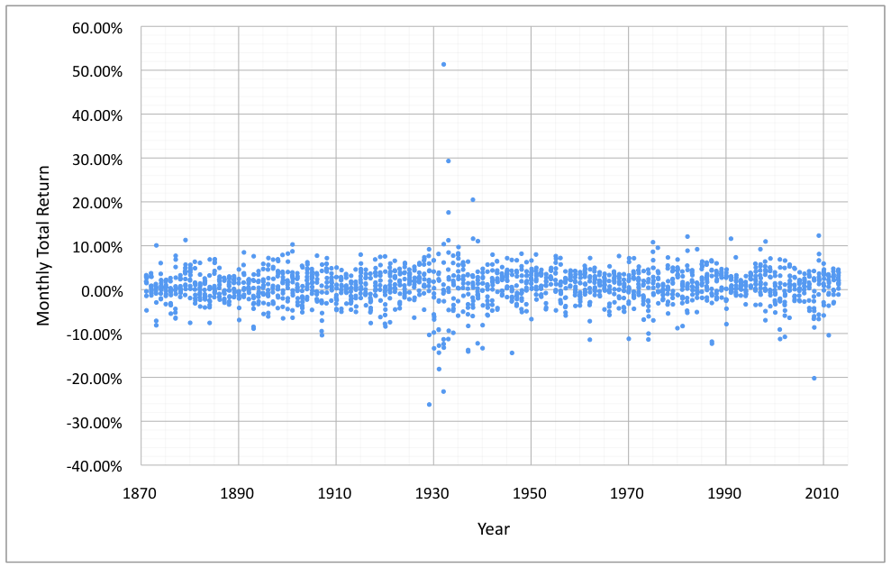
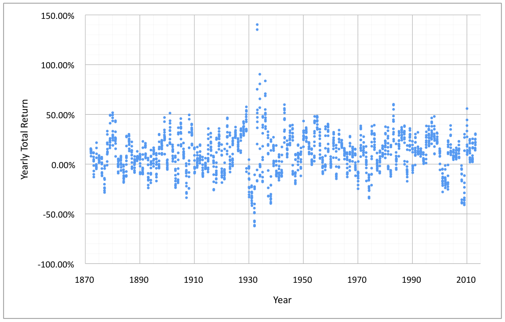
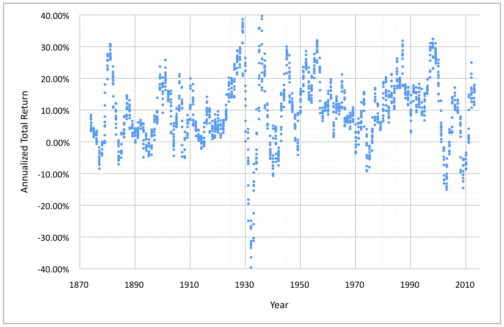
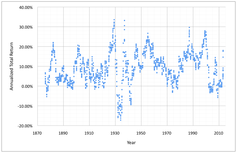
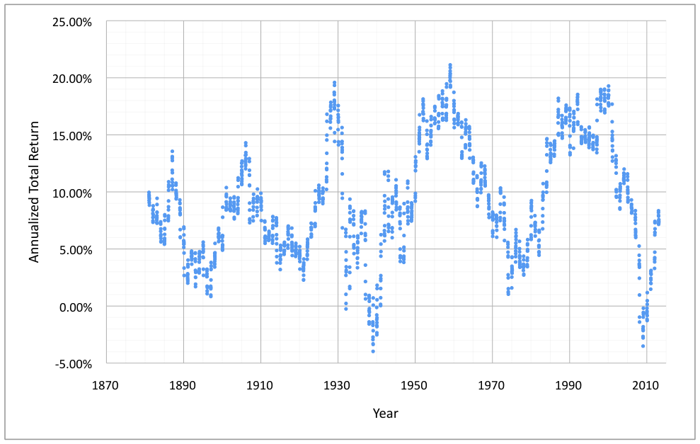
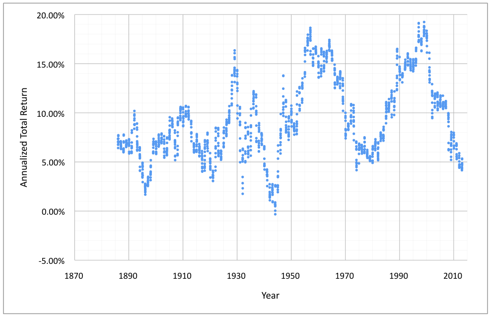
The first step in this analysis is to establish realistic rates of return for passive investors. Fortunately, Robert Shiller, a recent Nobel Laureate, provides data on the S&P 500 from 1871 to present, which is available on his Yale University website (http://www.econ.yale.edu/~shiller/data.htm). From this data, the charts below begin with historic one month total returns followed by rolling 1, 3, 5, 10, 15, 20 and 25 year returns calculated on a monthly basis (and hence there are 12 points on the graph for each year), and conclude with historic dividend yields on a monthly basis. Note that all of these graphs and histograms show the data prior to taxation.

—12.5% —10.0% —7.5% —5.0% —2.5% 0.0% 2.5% 5.0% 7.5% 10.0% 12.5%

0% 1% 2% 3% 4% 5% 6% 7% 8% 9% 10% 11% 12% 13% 14% 15% 16% 17% 18% 19% 20%

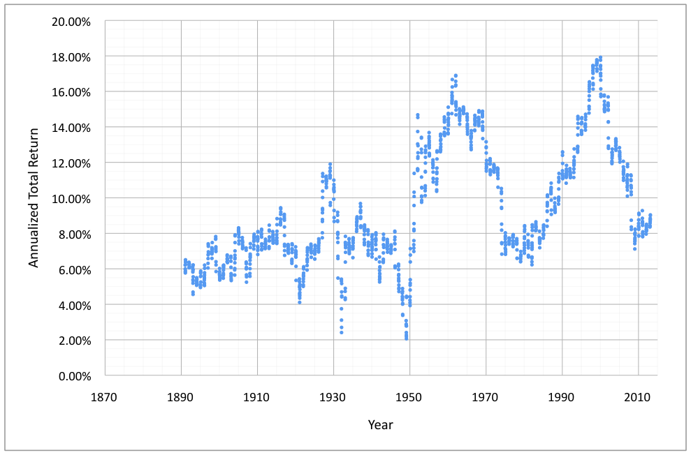
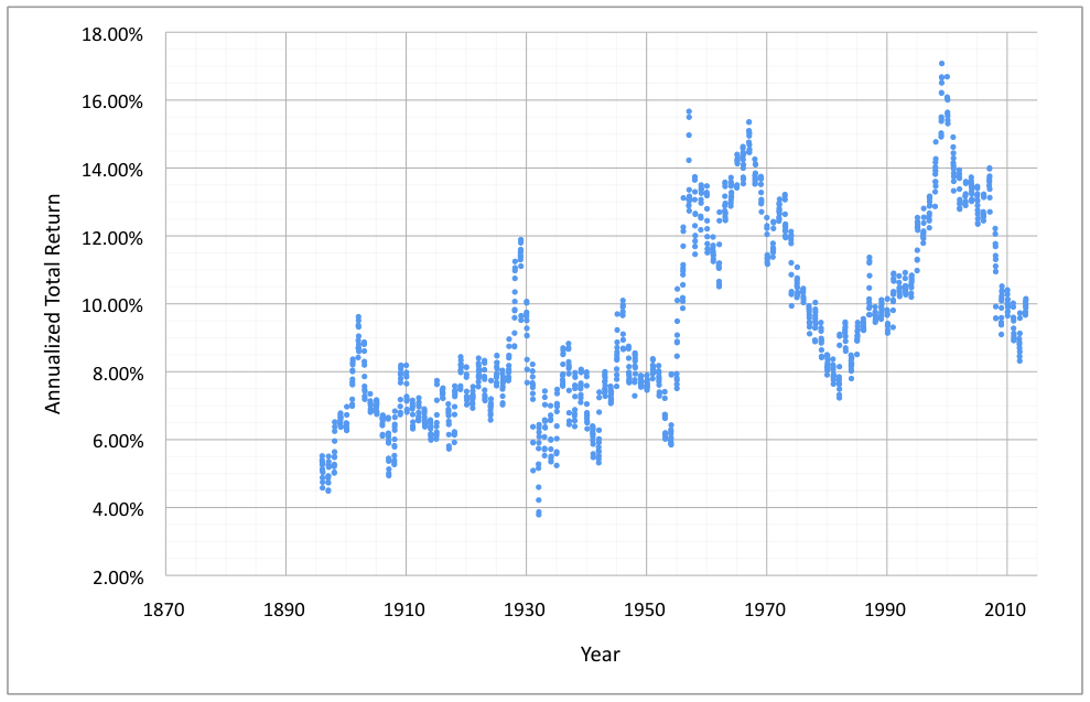
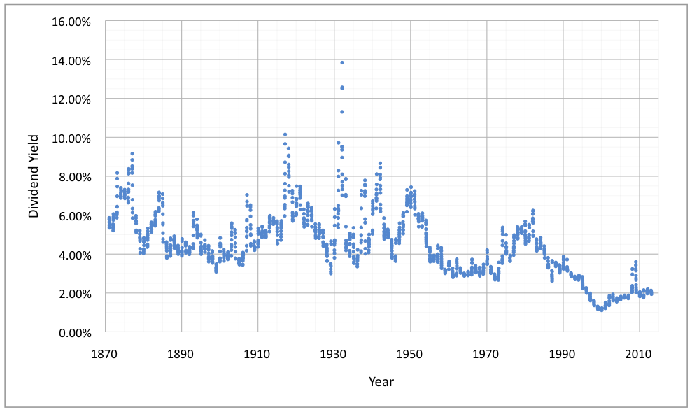
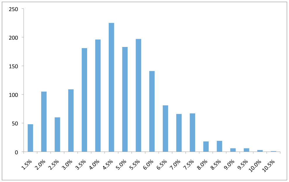
As can be seen, the historical dividend yield has varied between 1% and 8%, with a trend toward a lower dividend yield in the last few decades. Additionally, although long—run averages for stock market returns show a 9.3% annualized return, it is clear that there is quite a lot of variation, even at the 25—year level. However, from this data, the vast majority of returns fall between 0% and 20% for investment periods greater than three years.

Modeling Required Outperformance for Active Investing

Having determined realistic scenarios for passive investors, several variables can be considered to develop a model to calculate the required outperformance that an active investor must achieve to “break even” with a passive investor. As explained above, the required outperformance is calculated after fees and expenses, and thus applies to the net returns (after all fees and costs, but before taxes) of active and passive investors. As an aside, if the results were compared on a gross basis (before fees and taxes), the required outperformance would be even greater, as most actively managed funds have a much higher management fee than their passive counterparts. However, as most active investors report their results after fees and costs, and because these fees and costs vary from fund to fund (or manager to manager), this essay only takes into account returns after they have been deducted.

Perhaps the best approach for determining the appropriate variables to model is to describe the life of an investment. Initially, an investor makes a purchase: an index fund for a typical passive investor, or an actively managed fund for a typical active investor (if the investor actively selects individual stocks himself, then he can be considered a zero fee actively managed fund). Each year, both investors will receive dividends, which may generally vary between 1% and 8%, although in more recent times a typical dividend yield for an average selection of stocks is less than 4%. Additionally, each year there will be some amount of portfolio turnover where some portion of the portfolio is sold and invested into new stocks. There will likely be a very wide difference in turnover between the index fund of the passive investor and the actively managed fund of the active investor. In particular, the only real turnover for the passive investor will be index fund rebalancing, where the index fund periodically removes some companies from the index and replaces them with new ones 1 . For the active investor, the amount of turnover will generally depend on his or his fund manager’s investment time horizon and patience level. For both dividends and capital gains, both passive and active investors will be taxed, reducing their after—tax returns. For the purpose of this essay, capital gains distributions are modeled as being taxed at long—term rates, although this may not be the case for some actively managed funds. Under this assumption, both the dividends and the capital gains are modeled as being taxed at 20%, which is a typical taxation rate in the current environment. Finally, at some point, the investors will sell their shares of the fund and will be taxed on all unrealized gains up to that point. The time period from the

1 Turnover for an index fund varies from year to year, but is typically in the 3—5% range, implying a 20+ year holding period. However, in recent years, due to the fact that the market has generally been flat over a significant period of time (e.g., from the top of the Internet bubble to the Financial Crisis), increasing amounts of capital flowing to index funds, and the tax efficient structure of ETFs, index funds have been able to avoid distributing capital gains to investors. For example, the Vanguard Total Stock Market Index Fund has not distributed any capital gains since 2000. However, it is not clear whether capital gains distributions can be avoided indefinitely going forward, so the present model compromises by assuming a 1% turnover that is actually taxed, representing a compromise between no taxes and taxation on the full 3—5% turnover.

initial purchase to this selling point is defined as the “investment period” for this essay. It is only at this sale that the after—tax returns of the passive and active investor can be compared.

Important Variables

Thus, using the timeline above as a guide, the variables that are important for this comparison include:

1. The investment returns over the investment period . In particular, the higher the investment returns, the more the active investor will have to outperform the passive investor. For example, if the returns are 0%, then there is essentially no taxation of the gains, and as a result, no difference between the active and passive investor’s pre— and post—tax returns. However, with positive investment returns, the difference in taxation requires higher outperformance by the active investor. As investment returns increase, the required outperformance of the active investor correspondingly increases.

2. The turnover rate . The turnover rate for the active investor causes a tax burden for the active investor that is much higher than for the passive investor. This increased tax burden is the reason that the active investor must otherwise outperform the passive investor just to achieve the same after—tax results. Thus, the higher the turnover rate for the active investor, the higher the required outperformance.

3. The investment period . Generally, the longer the investment period, the higher the required outperformance for the active investor.

4. The dividend yield . Since dividends cause taxable events, the more the total return of the passive investor is caused by dividend yield, the lower the required outperformance of the active investor. At the extreme, if the entire total return is provided by dividends and both the passive investor and the active investor have similar pre—tax returns, they will also have similar post—tax returns, assuming the same dividend tax rate.

5. The tax rate . The higher the tax rate, the higher the required outperformance for the active investor.

Variable Values

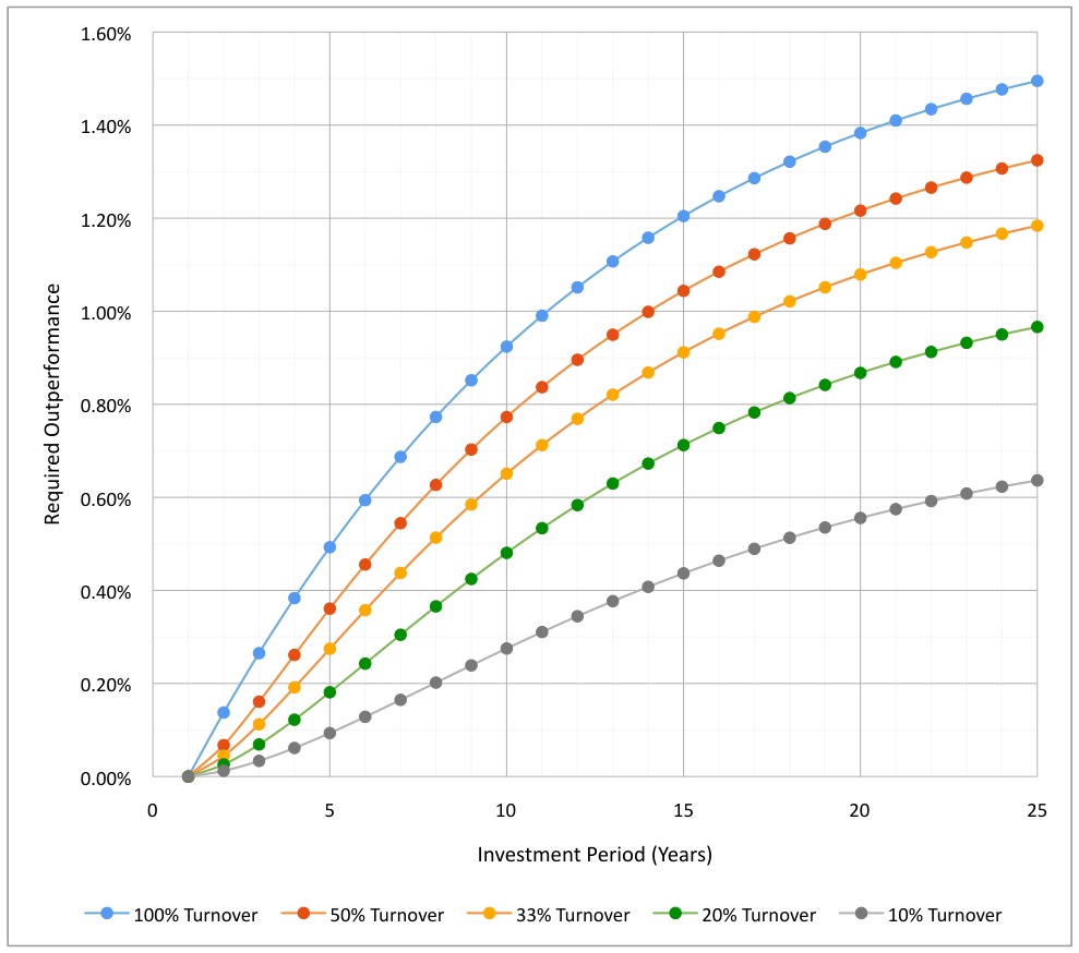
In the graphs below, the values of these variables are modeled as follows:

1. Investment returns of 5%, 7.5%, 10%, 12.5%, 15%, 17.5%, and 20% are shown in different graphs. These returns are based on the historic returns shown previously as well as the fact that a low investment return (e.g., less than 5%) results in very little required outperformance between the passive and active investor.

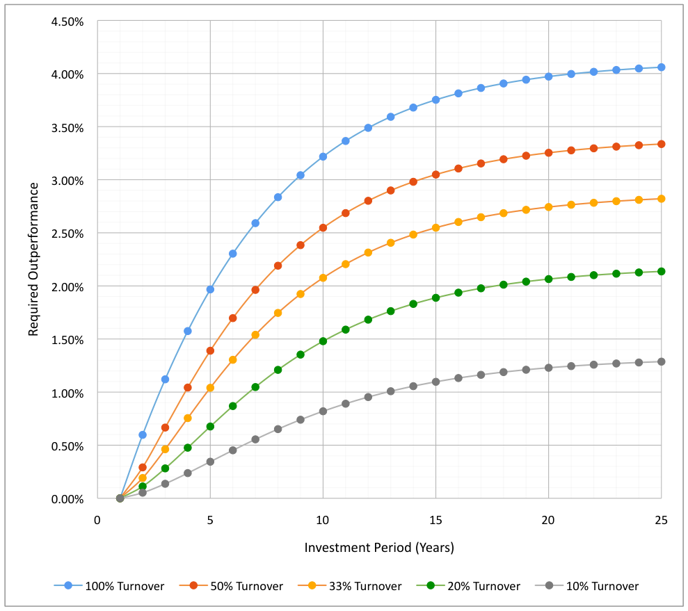
2. Turnover rates of 100% (implying an average single—year holding period), 50% (implying an average two—year holding period), 33% (implying an average three—year holding period), 20% (implying an average five—year holding period), and 10% (implying an average ten—year holding period). See the previous footnote for assumptions for the passive investor.

3. Investment periods of 1 to 25 years.

4. Dividends of 2.5% for both passive and active investors, based on recent dividend yields.

5. A tax rate of 20% on both dividends and capital gains, based on the current tax environment.

Modeling the Variables

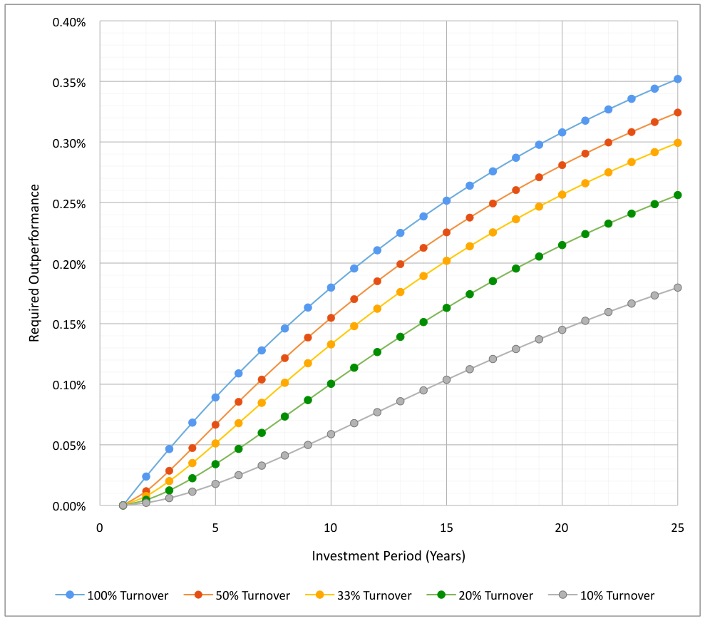
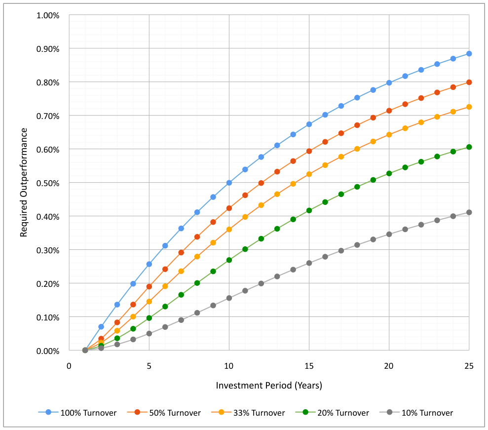
The following graphs illustrate the results of modeling the above values for the variables. To use them:

1. Select a desired pre—tax, annualized total return of a passive fund as the starting point for the comparison (e.g., the S&P 500 index). This step selects which of the following graphs are appropriate. For example, to compare the results of an active investor to an index over the last 10 years, select the graph corresponding to the annualized return of the index over the last 10 years.

2. Select the investment period. If this is retrospective, e.g., for determining if an active investor has outperformed the market after taxes, then simply select the desired investment period for the active investor. This step selects the X coordinate on the chosen graph. Following the example above, the X coordinate would be 10.

3. Determine the approximate turnover rate for the active investor. This step selects which of the lines within the selected graph is most appropriate.

4. Confirm that the assumed dividend yield and tax rate are appropriate for the current comparison.

5. Confirm that there are virtually no short—term gains from either the active fund or the passive fund. A discussion of the effects of short—term gains on required outperformance can be found following the graphs in the present essay, as well as in my previous essay “Holding Period, Taxes, and Required Performance”.

6. Using the selected graph, selected turnover rate line, and selected investment period on the horizontal axis, determine the required outperformance represented by the vertical axis. Adjust this required outperformance up or down to compensate for differences between the assumed pre—tax total returns and turnover rate and the actual values. Note that this is the required outperformance the active investor must achieve on a pre—tax basis (but after all fees and transaction costs) to match the returns of the passive investor.

7. Determine if the active investor outperformed the passive fund by adding the required outperformance to the pre—tax total returns of the passive fund and comparing the resultant value to the active investor’s returns.

Of course, the graphs below do not cover all possible scenarios for the above variables. However, it is relatively easy to use these graphs as a framework to assess virtually any long—term scenario, merely by interpolating among values in the provided graphs. For example, assume you desire to evaluate a 9% total return for the S&P 500 over a 10—year period for comparison with an active manager having a turnover rate of 25%. The closest graph is the 10% graph and the turnover line of 20%, which results in a required outperformance of 0.48%. This number should be adjusted down to account for the lower return (9% instead of 10%) and be adjusted up to compensate for the higher turnover rate—the actual

number happens to be 0.45%. Thus, the active manager should have returned 9.45% to have equivalent after—tax performance to the index fund over that period of time.

Caveats

One major caveat to this model is that it does not consider any tax—loss harvesting, where an active investor may sell positions with losses in order to offset corresponding realized gains from other positions, thereby reducing his tax burden. Accordingly, depending on the degree to which this strategy is successfully used, the required outperformance shown in the graphs may be overestimated. However, because this strategy’s use varies significantly from investor to investor, analysis at an individual level, rather than in aggregate (as in this model), would be required.

Considering Holding Periods of Less than a Year

In my prior essay, “Holding Period, Taxes, and Required Performance”, the effects of average holding periods of less than a year resulted in a much higher hurdle – a dramatic increase in required pre—tax returns, as compared to investments with average holding periods greater than a year. For example, to achieve a 15% after—tax return with an average holding period of less than a year and a 39.6% marginal tax rate, a 24.83% pre—tax return would have to be generated. In contrast, to achieve a 15% after—tax return with an average holding period of three years, only an 18.19% pre—tax return is required. From these findings, it would naturally follow that the required outperformance for active investors having average holding periods less than a year, or with greater than 100% turnover, would also be significantly greater than active investors having holding periods of greater than a year. However, rather than attempt to model such high turnover portfolios, which would require such an extensive set of assumptions as to be potentially useless, I elected to simply screen for a basket of funds having portfolio turnover in excess of 100% using Morningstar’s Mutual Fund screener 2 . From this screen, I compared the differences between pre— and post—tax results to that of the 100% turnover portfolio shown above, at the appropriate levels of return. As expected, there was a wide variance in the degree of difference between pre— and post—tax returns, but in most cases, the difference was significantly wider than those in the 100% turnover portfolio. In some cases, the difference increased the required outperformance by a full percentage or more, even at the three—year investment period level. However, there were also cases, particularly for periods spanning through the Financial Crisis, where the difference was similar to that of the 100% turnover portfolio. Presumably, these lower than expected differences result from tax loss harvesting during the period, which are not accounted for in the models of this essay. Thus, while I tend to believe that greater than 100% turnover has a significant impact in required outperformance due to short—term capital gains taxation, it is difficult to make any steadfast conclusions, and analysis on the individual fund level is generally required.

Establishing the Hurdle for Active Investors

In order to justify active investing in a taxable account, the active investor must be able to outperform an appropriately selected passive investment vehicle on an after—tax basis. Accordingly, not only must the active investor be able to consistently beat the appropriate passive investment in the commonly reported pre—tax results, he must beat it by an additional margin resulting from the additional taxes incurred by being active. The models shown in this essay allow an investor to determine the approximate value of this hurdle for the active investor under various scenarios. Perhaps more importantly, this essay provides a framework for the investor to rationally and honestly assess whether passive or active investing is the appropriate vehicle, depending on the investor’s skill level and expected returns.

2 For reference, according to various reports, Mutual Funds have average turnover rates of between 65% and 120%, depending on whether the turnover is asset weighted or not. Additionally, some reports indicate that hedge funds have turnover rates between 20% (lower quartile) and 50% (upper quartile) per quarter .