Puts and Takes

Dealing with price declines, particularly rapid ones, is one of the more difficult aspects of portfolio management. An ideal solution allows an investor to stay invested in good times and limit downside as well as take advantage of low prices in bad times.

Hedge funds attempt this feat by having a high exposure (sometimes over 100%) to ‘long’ positions while maintaining a significant portion (usually less than 100% which may be matched to the long portion greater than 100%) for ‘short’ positions. In good years, the long positions allow for positive returns (though they are generally expected to be less than the market), and, in bad years, the short positions protect the portfolio from large drawdowns (and is expected to allow returns to be better than the market). However, shorting is a particularly hard endeavor and includes the unenviable asymmetry of limited upside and unlimited downside.

Another solution is to hold a significant amount of cash, which decreases downside exposure and allows the investor to make purchases when low prices are available. However, as outlined in our prior essay “Why Hold Cash?”, the opportunity cost of the cash is generally expected to be worse than the benefit of deploying it at low prices, though this can vary from investor to investor.

Warren Buffett’s transition from fund manager to running Berkshire Hathaway allowed him to gain both permanent capital and the ability to reinvest cash flows. Access to a significant cash flow stream can be particularly useful in downturns, as the incoming cash can be used to invest in underpriced companies without any forced selling. However, even assuming a relatively high cash flow yield of 10%, only 2.5%- 5% of the portfolio might be available for deployment in a typical downturn.

This essay explores the possibility of using significantly out-of-the-money puts, bought at “cheap” prices, which may provide significant cash during a price drop at a relatively inexpensive price. Although there are caveats and downsides, this approach may be useful for some investors.

The Math of Options

Using a Black Scholes model, the inputs for valuing an option are: the underlying stock price, the strike price, the implied volatility, the risk free rate, the dividend yield of the underlying stock, and the expiry date. For the purposes of this essay, only puts are discussed, the dividend yield and risk free rate is held constant at 0% and 1%, respectively, and the expiry date is generally calculated at one year. Accordingly, the focus is largely on put price changes based on the underlying stock price and the implied volatility. In other words, throughout this essay, many of these variables are held constant in order to focus on the effect of underlying stock price and implied volatility.

A Simple Mental Model

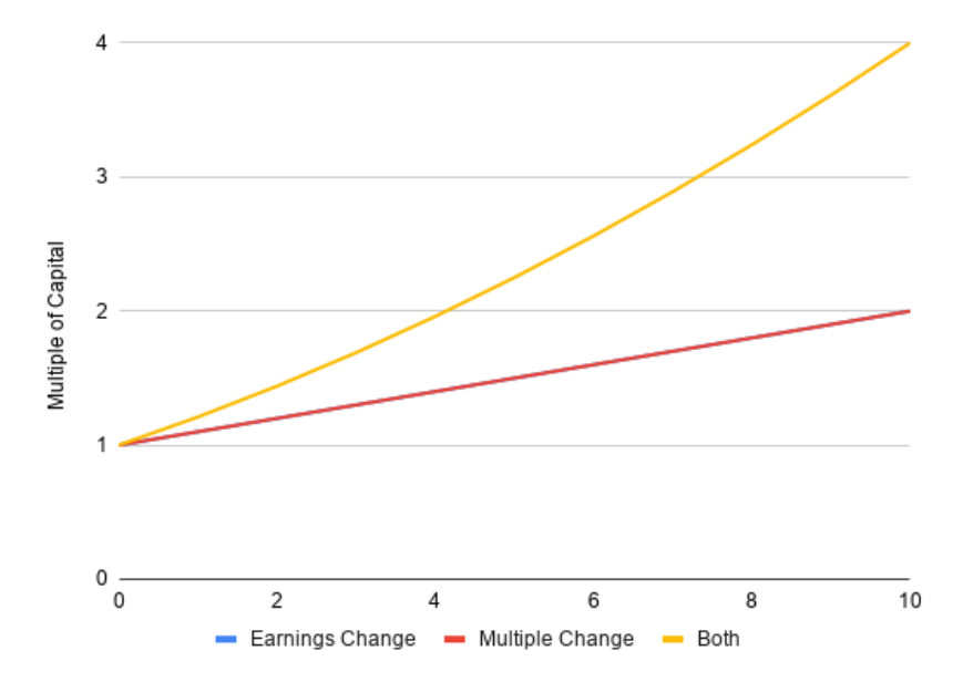
One simple way of thinking about the pricing of an option is analogous to the relationship between stock price, earnings per share (or some other fundamental metric), and the multiple of earnings.

An investor will do well when buying a stock at a relatively low multiple and the company’s earnings increases without a change in multiple—in this case, the investor’s gains are identical to the increase in earnings. Alternatively, an investor will also do well when buying a stock at a relatively low multiple and

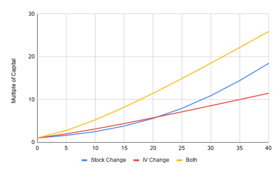
the multiple increases even when the company’s earnings do not—in this case, the investor’s gains are identical to the increase in multiple. However, a lollapalooza happens when the investor buys at a low multiple and both the underlying earnings increase and the multiple changes; for example, if the earnings double and the multiple doubles, the investor gets a 4x return instead of only a double in either case. The graph below shows how the returns look for each case as the earnings doubles and/or the multiple doubles (noting that the earnings change and multiple change exactly overlap).

Holding the expiry date constant, the price of an option is largely based on its intrinsic value (the amount of money that would be obtained if the option were exercised immediately) and its implied volatility. Using a simple analogy, the intrinsic value of the option can be compared to the earnings per share and the implied volatility can be compared to the multiple. An investor will do well when buying an option at a relatively low implied volatility and the intrinsic value increases (via a change in the underlying stock price) without a change in implied volatility—in this case, the investor’s gains are effectively the change in intrinsic value. The investor will also do well when buying an option at a relatively low implied volatility and the implied volatility increases without a change in the underlying stock price—in this case the investor’s gains are based on the increase in the implied volatility. Somewhat similar to the earnings and multiple example above, when an investor buys an option at a low implied volatility and both the implied volatility increases with a change in the underlying stock price, significantly better returns can happen. However, the relationship between the option’s price and intrinsic value and implied volatility are not as straight-forward as the earnings example above because the impact of implied volatility is higher when the strike price and underlying price are close to each other and lower when the strike price and underlying price are further away from each other.

Expected Volatility

Before showing the relationship between put prices and changes in the underlying stock price and implied volatility, it is important to establish typical ranges for these parameters and their relationship with each other. The following table indicates the frequency, within a calendar year, of drops from peak to trough for the S&P 500 from 1979-2020:

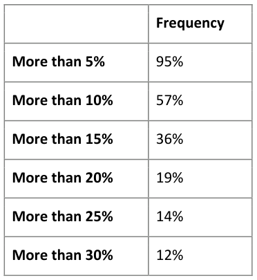
Thus, investors should expect corrections of more than 10% to happen quite often (e.g., every 1-2 years) and drops of 20% or more around every 5 years.

Implied volatility generally moves upward in lock-step with price declines and usually rapidly. Looking at implied volatility from 1990 on, in ‘good’ times, when investors are not concerned with significant events, implied volatility may generally range between 10 and 20. When price declines of more than 10% (but less than 20%) occur, implied volatility generally moves upward and can range between 25 and 40. When price declines of more than 20% (but less than 30%) occur, the implied volatility can range between 30 and 50. Price declines of more than 30% are generally associated with implied volatility of greater than 40, reaching as high as 79 in 2008 and 66 in 2020.

Example Returns of Puts

As noted above, the relationship of put returns with underlying stock price declines and implied volatility changes is similar to (though not as straight-forward as) the relationship between stock prices with earnings and multiple changes. The following graphs illustrate examples at different initial implied volatilities, strike prices, and price declines.

At the Money

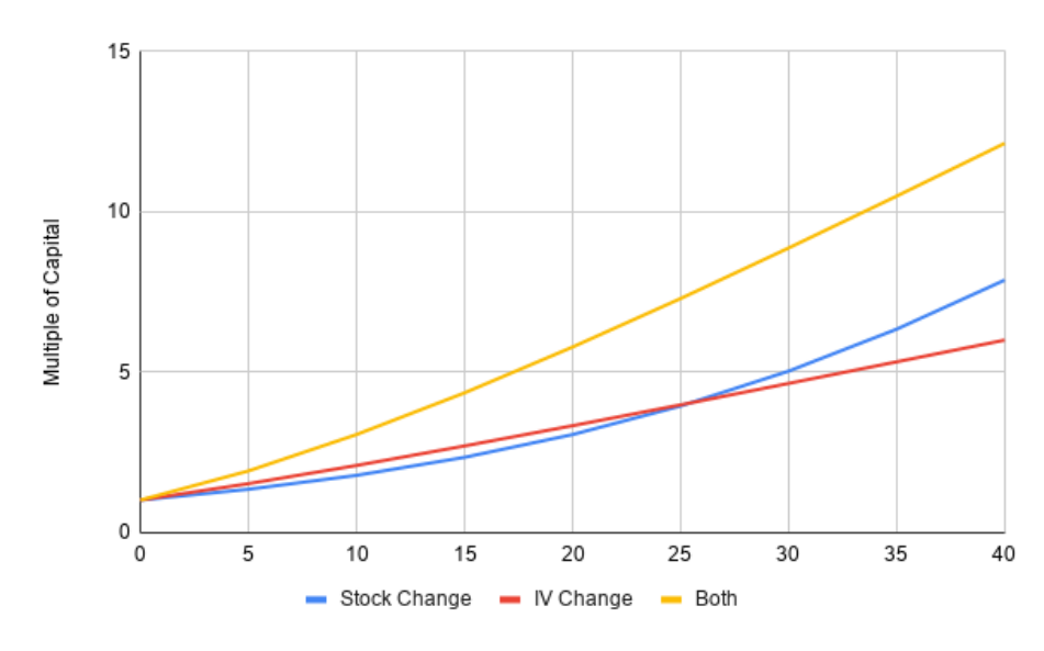
As an initial example, the following graph shows this relationship when an investor buys a put with a strike price at the money (meaning the strike price is the same as the current underlying price) with the following conditions: 1) stock price drops as much as 45% (indicated by the 0-45 change in the graph); 2) implied volatility increases from 15% to 60% (also indicated by the 0-45 change in the graph); or 3) both.

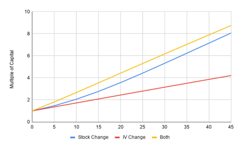
While the multiples of capital appear to be impressive in this example, as compared to later examples, the gains are relatively modest given the large movement in stock price and implied volatility. Additionally, while the implied volatility change has some impact, the stock price change is substantially what drives the gains.

Out of the Money

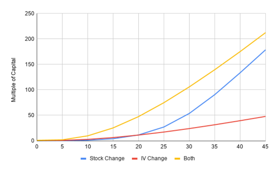
However, if an investor buys a put option with a strike price 25% out of the money in the same conditions, the outcome is quite different.

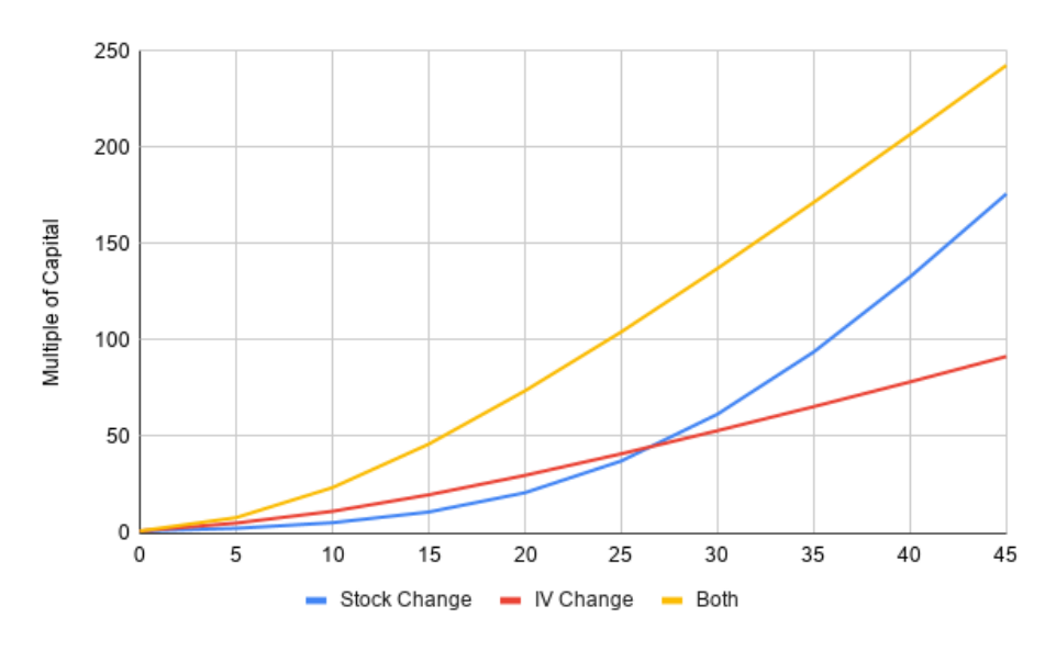
As shown, the potential multiple of capital is orders of magnitude larger than the at the money case. Additionally, a true lollapalooza effect happens in the out of the money case, where the combination of stock price change and implied volatility change is bigger than a simple addition of the two individual cases.

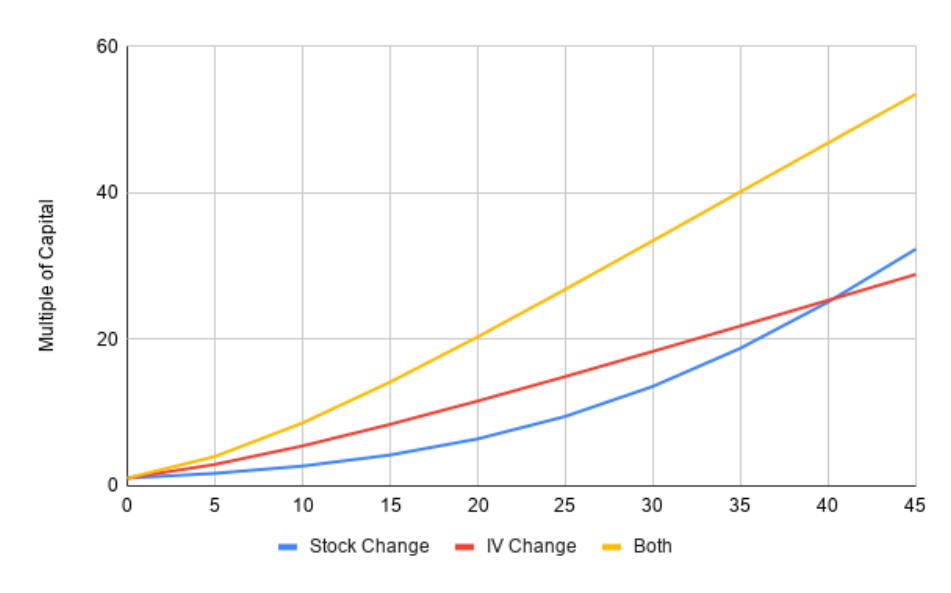
This effect also works with a higher implied volatility start (e.g., 20%) and a lower (but still significant) drop in stock price (e.g., 40%).

As shown, the returns are still much better than the at the money case, but significantly worse than the 25% out of the money case.

Elevated Implied Volatility

If an investor buys at an elevated implied volatility (e.g., 30%), with a 25% out of the money put, and implied volatility spikes as high as 70 (e.g., as it did 2009 reaching 80 and nearly did in 2020) while the stock drops 40%, the returns are not as good.

Longer Dated Puts

If an investor buys longer dated puts (e.g., 2 years), returns are reduced. The following graph shows the exact scenario of 25% out of the money, except with 2 years:

As shown, the longer date causes a very large reduction in returns, relative to the 1 year case.

Conclusions - Proposed Rules of Thumb and a Laundry List of Caveats

First, the caveats—the graphs above are not to be used for prospective returns, because several of the assumptions will not hold. For example:

1. The expiry date was held constant at 365 days in all but the last example above and thus shows the returns if all of the changes happened on day 1. However, downturns and volatility spikes may occur at any time during the period of the put (or might not occur at all). Accordingly, there is a fair amount of option value that decreases over time that is not represented well in the graphs. For example, the multiple of capital for the 25% out of the money case decreases (but remains high) if the drop happens half-way through the option period.

2. A related issue is that stocks generally go up over time, so unless the price decline occurs near the price when the put was bought, the decline relative to the initial purchase time may be significantly smaller than what is shown in the various graphs above. For example, if an investor buys a put when the index is at a value of 100, and the index increases to 125, followed by a 40% decline to 75, the comparable decline would only be 25% for the investor (relative to the initial 100 price). Saying this another way, using the graphs in this essay, the investor would only get the gains associated with the 25% decline, rather than the 40% decline. 3) The graphs also assume that the options are actually available at these calculated prices, which may not always be true and/or may significantly change the multiple of capital. For example, depending on the amount of puts to be purchased, there may simply not be enough liquidity (particularly at 25% or more out of the money levels) to be purchased. It is worth noting that this problem does not occur when the put gets close to the money, in which case, liquidity will increase significantly. 4) Alternatively, or additionally, there may be liquidity, but the prices may be higher than expected.

As an example, the 25% out of the money case, at 15% implied volatility, with a 1 year expiry date is calculated as $0.11. If the actual price was, for example, $0.22, then all of the multiples would need to be divided by two in the graph above. 5) There is also a significant issue related to when to sell the options, which is that it is very hard to know when the market has stopped dropping or implied volatility has stopped increasing. If an investor sells too soon, then the value has not been maximized. On the other hand, sometimes the price drop and volatility returns back to prior levels very quickly, so all of the ‘gains’ may be lost.

6. Psychologically, it is difficult to buy these options year after year, as in general they will expire worthless and represent a headwind to performance most of the time. On the other hand, they are amazing when they work!

Some Proposed Rules of Thumb

First, the most important rule is to make sure the price of the option is as low as possible. For example, for a one-year expiry, the put should cost less than 1% (and hopefully significantly less) of the underlying stock price. Thus, for a stock of $100, an investor would want to pay less than $1 for the put. This price can mostly be achieved by buying at an implied volatility that is 20% or less and with a strike price that is 20% or more out of the money. For puts that cost significantly more than that, the returns stop being asymmetric and may not pay off over time, given the general expectation that the market will go up.

Second, the further out of the money the put is, the lower the price, and generally, the better the returns are expected to be for any significant downturn. As noted in the caveats above, the major problem is likely liquidity as most options trade closer to the money.

Third, the returns for one year options appear to be significantly better than two year options, but this has its own downside as the prices of options change over time (e.g., implied volatility changes quite often), so a ‘cheap’ option may not be available the next year. An alternative solution is to buy two-year options and roll them each year, but the returns are generally lower and there is significant decay in extrinsic value over time. For example, a put purchased 25% out of the money at two years is worth about 1/3 as much a year later, with no change in price (which is generally expected to go up, decreasing the put’s price even more).

Finally, the rules of thumb for selling are difficult. A general trader’s rule of thumb is to sell 1/3 on every triple; however, this strategy is not particularly viable for these types of puts because the implied volatility and the price drops usually happen quickly. For example, for the 25% out of the money case with 15 implied volatility, after a 10% correction, the multiple of capital is already 23x! A more general rule would be to continuously sell portions of the put as it appreciates and fully sell when the underlying index drops more than 35% and implied volatility of more than 60% is reached.